The End of the NEC Era: Why AN-SOF is the Only Modern Engine for 2026 and Beyond
For decades, names like EZNEC, 4NEC2, and MMANA-GAL have been the “standard” in antenna modeling. However, as we move through 2026, a critical reality has set in: The era of NEC (Numerical Electromagnetics Code) is over. While these programs are still widely discussed online, most users are unaware that they are working with abandoned interfaces and 50-year-old math that no longer receives support or updates. If you are looking for accuracy, reliability, and active development, there is now only one living contender in the field: AN-SOF.
The Illusion of “Standard” Software
A common misconception is that EZNEC or 4NEC2 are simulation engines. They are not. They are merely User Interfaces (UIs) that run various versions of the NEC engine developed at Lawrence Livermore National Laboratory (LLNL).The state of these tools today is stark:
- EZNEC: Discontinued in 2021. The developer has retired, and the software is provided “as is” with no future updates.
- 4NEC2: Has not seen any updates since 2021.
- MMANA-GAL: Essentially frozen in time since 2009.
The NEC Development Dead End
The evolution of the NEC engine itself has reached a full stop. G.J. Burke, the lead developer at LLNL and the primary mind behind NEC-2 and the later NEC-5, passed away in 2021. With his passing, the internal expertise required to update or fix the deep-seated architectural issues in NEC has vanished. While LLNL continues to sell licenses for NEC-5, they provide no technical support or ongoing development.
Why NEC Engines Fail Modern Requirements
Even at their peak, the various versions of NEC were riddled with mathematical “ghosts” and physical limitations that engineers have had to “work around” for decades:
- NEC-2: A 1970s Relic. This 1981 release persists primarily due to its “abandonware” status rather than technical fidelity. The engine relies on the thin-wire approximation, which assumes current is a filamentary flow along the wire axis. By neglecting the surface kernel, it fails to account for current distribution along the wire’s actual circumference, leading to significant inaccuracies in thick-wire structures or complex junctions. It suffers from 7 fundamental limitations, including kernel singularities and spacing constraints, which are addressed only by moving to a Conformal Method of Moments (CMoM).
- MININEC: Physically Incomplete. Developed at the Naval Ocean Systems Center (NOSC) for 16K-32K RAM systems, its heritage is one of extreme memory efficiency over physical completeness. While it is often praised for handling tapered wires more gracefully than NEC-2, it remains flawed for real-world modeling. It utilizes a Perfect Electric Conductor (PEC) model for input impedance, meaning it ignores ground losses at the feed point while simultaneously including them for far-field calculations. This contradiction results in misleadingly high efficiency reports that do not correlate with field measurements.
- NEC-4.2: Architectural Instability. Released in 1992, this version attempted to fix NEC-2’s limitations but was hamstrung by its rigid FORTRAN framework, resulting in internal errors that were never fully resolved. It relies on the point matching (collocation) technique, forcing the electric field to zero only at discrete points on the wire surface rather than along a continuous path. This method is inherently unstable for small loops and tapered elements, where the input impedance often fails to converge or exhibits non-physical oscillations.
- NEC-5: The Resonant Frequency Trap. This 2019 update introduced linear testing functions to improve upon point matching. However, the implementation forces a symmetry constraint that requires an even number of segments to model center-fed dipoles. This architectural quirk creates a permanent offset in the resonant frequency, forcing precision-focused engineers into a cycle of manual compensation rather than relying on the simulation’s raw data.
- The “Apex” and Spacing Problem. No legacy NEC engine can mathematically reconcile the “apex” problem found in sharp-angled structures like Inverted V antennas. When wires are spaced closer than a few wire radii, the thin-wire kernel breaks down, causing mutual coupling calculations to produce “ghost” values.
It is a common myth that MMANA-GAL is inherently more accurate than EZNEC or 4NEC2. In reality, these are merely User Interfaces (UIs). EZNEC supports up to NEC-5, while 4NEC2 is limited to NEC-4.2 and MMANA-GAL relies solely on MININEC. Curiously, while MININEC is more accurate for tapered wires, this is a result of its specific MoM formulation rather than the interface itself.
AN-SOF: The Living Alternative
Unlike the tools listed previously, AN-SOF is not a mere “wrapper” or graphical interface for legacy code developed in the 1970s. Since its debut in 2010, AN-SOF has been built upon a completely original computational engine: the Conformal Method of Moments (CMoM).
While NEC-based tools have effectively become “abandonware,” AN-SOF is an evolving R+D+I platform. By moving beyond the limitations of the original LLNL source code, it eliminates the structural flaws inherent to the NEC era:
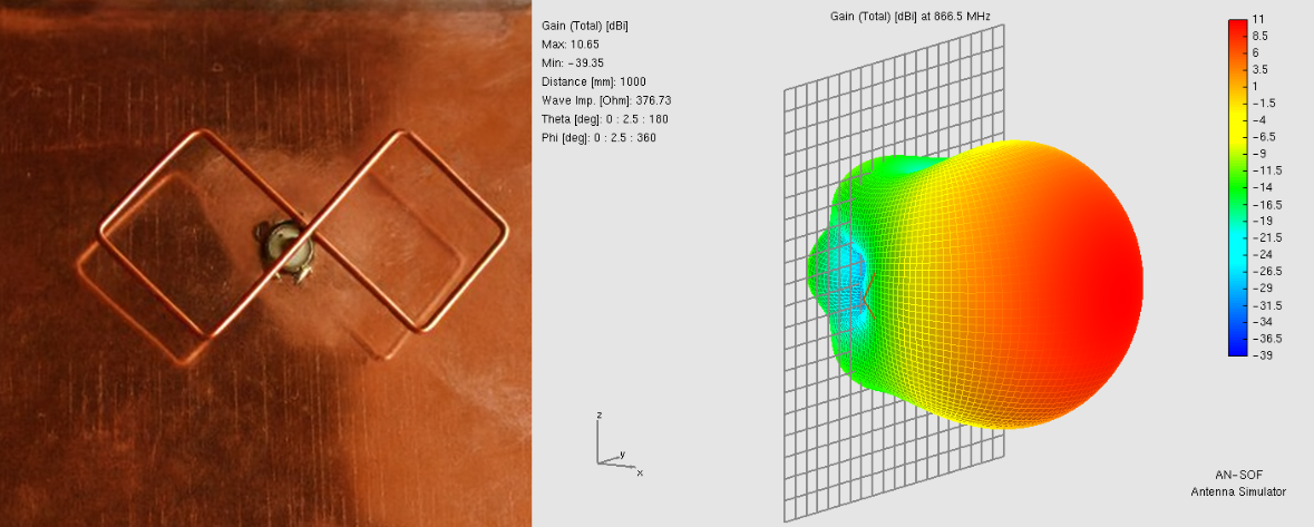
- Geometric Integrity and the “Bent Wire” Solution. Legacy engines often “guess” at the physics of acute angles, leading to the well-known “bent wire” error where the current distribution becomes non-physical at the junction. AN-SOF’s CMoM solver maintains mathematical stability at the apex of structures like Inverted V antennas, ensuring that the boundary conditions are satisfied exactly along the entire wire surface.
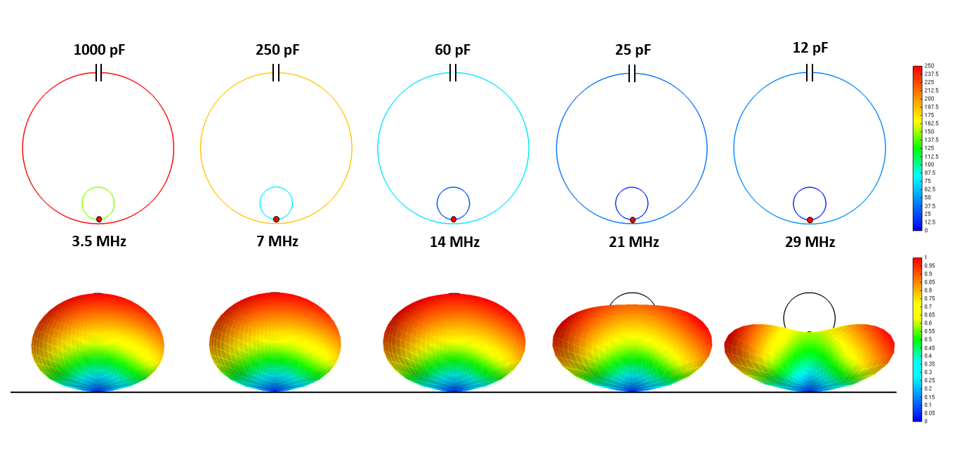
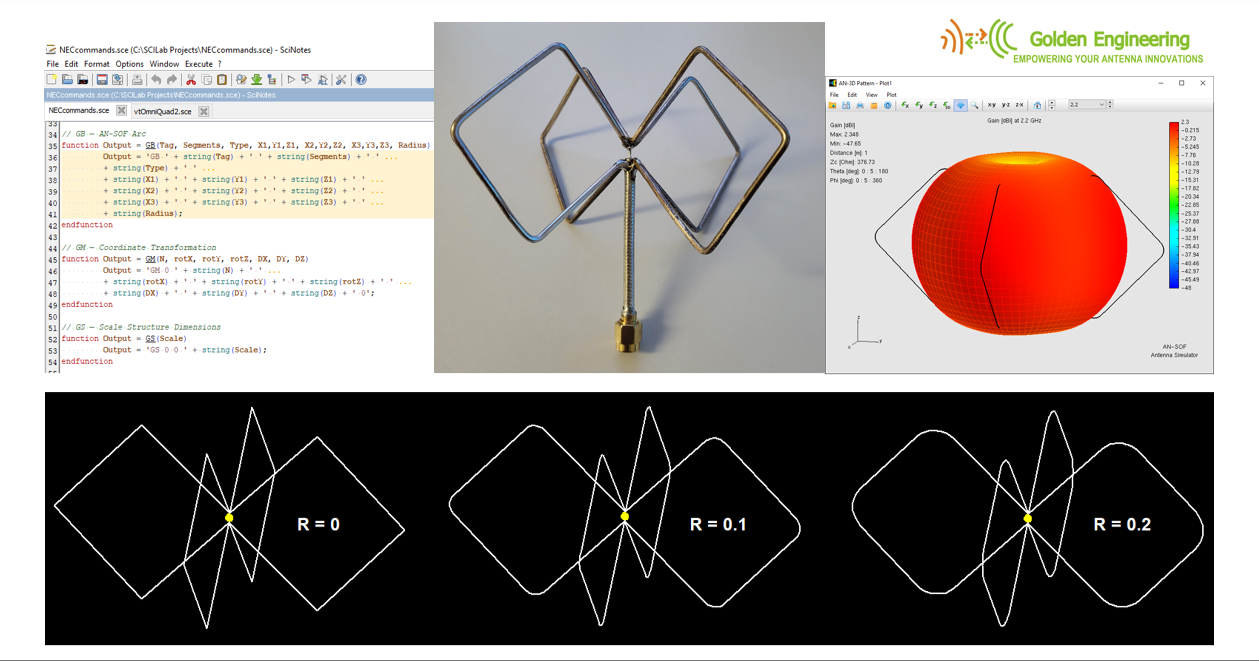
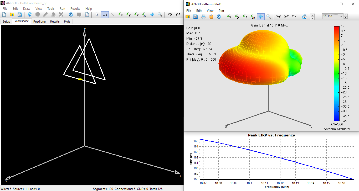
- True Curvilinear Modeling. For circular loops, spirals, and helices, AN-SOF utilizes curved segments that follow the actual physical geometry of the conductor. This is a significant leap over the legacy approach of using a “string of short straight segments,” which introduces artificial discretization errors and necessitates higher segment counts just to approximate a simple curve.
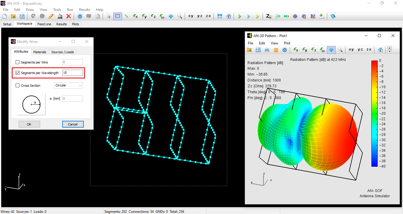
- The Exact Kernel vs. Thin-Wire Approximation. NEC engines rely on the thin-wire approximation, a simplification that assumes current flows only on the axis and breaks down when the wire radius $a$ is no longer negligible compared to the segment length $\Delta L$. AN-SOF utilizes the Exact Kernel, performing a full surface integration of the Green’s function. This allows for the simulation of “thick” wires and closely spaced elements with a level of precision that NEC simply cannot achieve.
- Physics-Based Ground Modeling (Sommerfeld-Wait). Most legacy tools utilize the Reflection Coefficient Approximation (RCA) for ground screens, a method that is only truly valid in the far-field. AN-SOF implements the rigorous Sommerfeld-Wait ground model. This exclusive implementation treats the lossy ground and radial wire screens as physical realities, providing accurate input impedance and near-field data where RCA-based tools provide only approximations.
- Expert-Driven R+D Support. In an environment where technical support for RF software is often relegated to community forums or dead links, AN-SOF offers a professional ecosystem. Users have direct access to a “Living Platform” supported by RF engineers, ensuring that the software evolves alongside modern engineering challenges.
Preserve Your Engineering Legacy: Direct NEC Import
Decades of antenna modeling have resulted in a massive global library of designs stored in legacy NEC formats. Transitioning to a modern simulation environment should not mean discarding years of refined models or starting from scratch. AN-SOF honors this engineering legacy by providing a seamless NEC import utility, allowing you to bring your existing designs into our advanced computational environment instantly.
By importing your legacy files, you can immediately upgrade your workflow from 1970s-era approximations to the high-precision Conformal Method of Moments (CMoM) engine:
- Zero-Effort Migration. You can import standard .NEC files directly into AN-SOF without manual re-entry of wire coordinates, radius data, or source placement.
- Immediate Accuracy Gains. Once imported, your existing geometry is processed by the Exact Kernel and the Sommerfeld-Wait ground model, providing a more rigorous physical analysis than legacy solvers.
- Advanced Post-Processing. Use AN-SOF’s modern toolkit to visualize 3D far-field patterns and analyze near-field EMF compliance on designs that were previously “locked” in text-heavy legacy formats.
Transitioning from EZNEC
For users migrating from the EZNEC ecosystem, we have streamlined the path to higher precision. You can export your descriptions and bring them into AN-SOF to leverage our specialized tools for R+D+I.
Download the Instruction Guide:
PDF: How to Export from EZNEC and Import into AN-SOF
Summary: The Choice in 2026
We are at a crossroads in antenna simulation. You can continue to use “relic” software that relies on the unsupported math of the 1970s and 80s, or you can move to a professional engine designed for the complexities of modern RF design.
AN-SOF stands alone as the only living, updated, and high-accuracy antenna simulation tool of its kind. For those who demand results that match real-world measurements, without the “ghosts” and computational artifacts of the NEC era, the choice is clear.
Request Your AN-SOF Trial Today: