Tuner for Impedance Matching

The Tuner Calculator

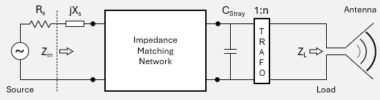
AN-SOF features a tuner calculator that enables impedance matching of an antenna input impedance, an antenna with a feeder already connected to its terminals, or a given custom load.

To access the tuner calculator, choose the Tuner tab in the AN-SOF main window (Fig. 1). Here, you can set the tuner parameters on the left side of the window and view the results on the right side. The tuner consists of three components, each of which will be described in the following sections:

• Impedance Matching Network: This component allows the synthesis of an impedance matching network based on the impedance seen at the network output and the desired impedance at the network input. The quality factors of the network, inductors, and capacitors can be adjusted to model real-world scenarios.

• Stray Capacitance: Some networks, particularly high-pass Tee networks, exhibit a parallel stray capacitance at the network output. This capacitance can be specified to account for this effect.

• Impedance Transformer: An impedance transformer can be specified at the network output to transform the input impedance of an antenna, the input impedance of a feeder connected to an antenna, or a custom load entered by the user.

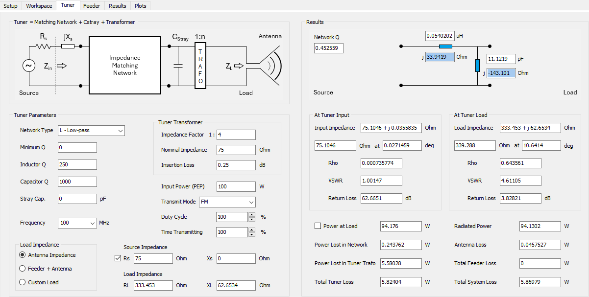
Impedance Matching Network

In the Tuner Parameters box, you can configure the impedance matching network, as shown in Fig. 2.

By expanding the Network Type dropdown menu, you have the following options:

• No Network: Select this option to bypass the matching network, making the network input impedance equal to the impedance at the network output.

• Based on the impedance seen at the network output and the source impedance connected to the network input side, AN-SOF can synthesize the following networks:
  • L – Low-pass
  • L – High-pass
  • PI – Low-pass
  • PI – High-pass
  • T – Low-pass
  • T – High-pass

The network components will be automatically calculated to match the source impedance (R_s + jX_s) connected to the network input side. If the source impedance has a reactance component, jX_s, the network will “absorb” this reactance so that the input impedance of the network plus jX_s will match the real part, R_s, of the source impedance. The same principle applies to the load impedance seen at the network output side. If the network load impedance has an imaginary part, it will be absorbed by the network to synthesize the network components (inductors and capacitors).

Note that a low-pass network could include series capacitors instead of inductors or parallel inductors instead of capacitors, depending on the complex impedances (with real and imaginary parts) being matched. Similarly, a high-pass network might involve series inductors instead of capacitors or parallel capacitors instead of inductors.

You can specify a minimum Q for the network synthesis calculations, as well as the Q for the inductors and capacitors. This allows you to account for component losses to represent real-world components. To model ideal zero-loss components, enter high Q values, such as 1E8.

Stray Capacitance

Stray capacitance, also known as parasitic capacitance, refers to unintended capacitance between two conductors separated by a dielectric or free space. This effect is particularly noticeable at the network output side when a transmission line is connected. AN-SOF allows for the configuration of a feeder composed of a transmission line to feed an antenna, enabling modeling of stray capacitance to accommodate this scenario. While stray capacitance is commonly observed in Tee high-pass networks, it can be added in any case. Typical values range from around 10 pF in HF bands.

Impedance Transformer

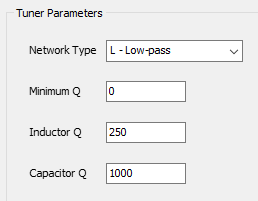
In the Tuner Parameters box, an impedance transformer, also known as a “trafo” in RF jargon, can be specified, as shown in Fig. 3.

The transformer allows us to divide a load impedance by a factor, n, making it a 1:n transformer. It’s important to note that this is the impedance transformation factor, not the voltage transformation factor, which is n^-1/2 and is determined by the primary-to-secondary winding relationship of a transformer. A transformer can be used to reduce a high impedance to approach the standard 50 or 75 Ohms used in transmission lines and RF devices. Both the real and imaginary parts of the load impedance will be divided by n.

If n is in the range 0 < n < 1, the transformed impedance will be higher than the load impedance connected to the output side of the transformer. A factor n = 1 can be used to model a 1:1 transformer, also known as an isolation transformer, which is used to transfer voltage from one electrical circuit to another and to isolate a powered device from the power source. The 1:1 ratio transformer has the same input and output voltage and current. It is used to protect secondary circuits and individuals from electrical shocks between energized conductors and earth ground. It also reduces voltage spikes in the power supply line caused by rapid changes in lighting, static electricity, or voltage.

Real-life transformers are manufactured for a specified nominal impedance transformation. The nominal impedance can be entered in the Tuner Transformer box, as well as the transformer insertion loss in decibels. Manufacturers specify a transformer insertion loss relative to a nominal impedance, so it is important to specify the nominal impedance as well. The insertion loss is defined as the power lost inside the transformer, measured in dB relative to the input power. Thus, the output power delivered by the transformer to the load impedance will be lower than the input power due to losses inside the transformer materials (coil conductor losses, magnetic core losses, etc.).

Tuner Frequency and Input Power

The components synthesized in the impedance matching network of the tuner will be automatically calculated for a specified frequency, which can be chosen from a dropdown menu in the Tuner Parameters box, as shown in Fig. 4.

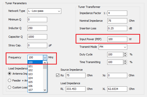
This list of frequencies is taken from the Frequency panel in the Setup tab, where a single frequency, a list of frequencies, or a frequency sweep can be configured. Therefore, to change the list of frequencies available in the Tuner tab, go to the Setup tab and enter the desired frequencies in the Frequency panel. Note that the frequency chosen for the tuner will be its design frequency; thus, the tuner components, inductors, and capacitors will be recalculated if the design frequency changes.

The Input Power to the tuner can also be specified in the Tuner Parameters box. This is the power delivered by the source connected to the input side of the impedance matching network of the tuner. This input power affects the powers calculated in the Results box on the right side of the Tuner tab, as explained below. It is worth mentioning that the tuner input power is not the power delivered to the antenna terminals, which can be set in the Excitation panel of the Setup tab. However, if the tuner is connected to an antenna, we can specify that the tuner output power be delivered to the antenna terminals, as detailed below.

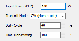
Transmit Mode, Duty Cycle, and Time Transmitting

The input power specified is the transmitter’s Peak Envelope Power (PEP). However, when performing RF exposure evaluations, the average power supplied by the transmitter over time is the critical factor. The average power is a fraction of the PEP, determined by the duty cycle (or duty factor) of the selected transmit mode. The transmit mode can be chosen, and the corresponding percentage duty cycle will be displayed, as shown in Fig. 5. To enter a custom duty cycle, select “Custom” as the transmit mode.

It is also important to account for the percentage of time the transmitter remains active within a specific period, such as 6 minutes. For example, if the telegraph mode transmits for only 3 minutes in every 6-minute period, the power considered for RF exposure calculations is reduced by 50%. Therefore, the Time Transmitting parameter can be set as a percentage. Both the duty cycle and the time transmitting percentage will affect the PEP, and an average input power will be calculated accordingly.

Tuner Source and Load Impedances

The source impedance connected to the tuner input side can be set in real (R_s) and imaginary (X_s) parts, as shown in Fig. 6.

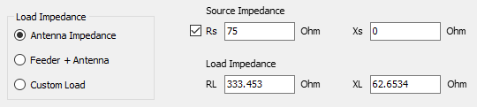
When a non-null source reactance, X_s, is entered, it will be absorbed by the impedance matching network calculations. Thus, the net input impedance of the network, after adding jX_s, will be matched to the real part of the source impedance, R_s. Click on the checkbox next to the “R_s” label to set this resistance as the reference impedance for VSWR calculations. This same resistance will be automatically set in the Settings panel as the “VSWR Ref. Impedance”.

There are three options for the tuner load impedance (R_L + jX_L):

• Antenna Impedance: Select this option to set the antenna input impedance as the tuner load. Note that the antenna impedance varies with frequency, so changing the design frequency for the tuner will trigger a recalculation of the impedance matching network.

• Feeder + Antenna: This option allows us to set the combination of feeder + antenna as the tuner load. In this case, the feeder parameters will be taken from the Feeder tab at the chosen design frequency. Therefore, the load impedance connected at the tuner output is a function of frequency since it is the input impedance to the feeder connected to the antenna.

• Custom Load: This option allows setting a tuner load impedance manually by specifying its real (R_L) and imaginary (X_L) parts. The Tuner tab can be used as an independent impedance matching calculator in this case.

Tuner Results

The results of the calculations based on the configured tuner parameters are displayed in the Results box on the right side of the Tuner tab, as shown in Fig. 7.

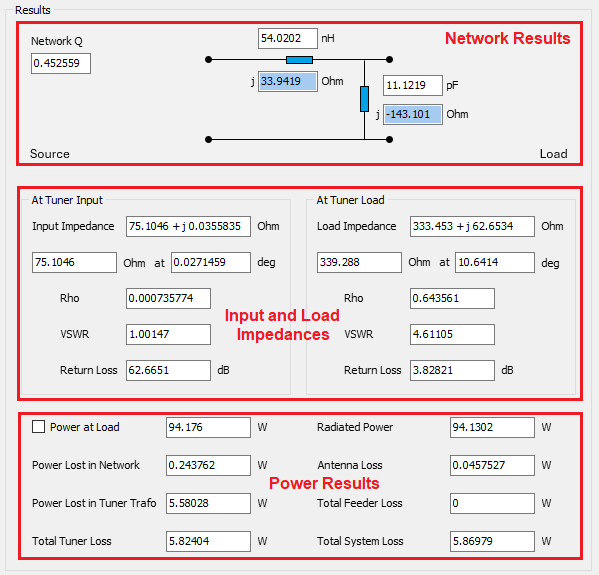
The results are categorized into three sections: Network results, input and load impedances, and power results.

Network Results

The network results shown include the resulting network Q and a diagram illustrating the network components, including inductors and capacitors. For inductors, their inductance in Henry and reactance in Ohms will be displayed, while for capacitors, their capacitance in Farads and reactance in Ohms will be shown. The units of inductance and capacitance displayed can be changed to pH, nH, uH, mH, H, or pF, nF, uF, mF, F, respectively, by navigating to the AN-SOF main menu > Tools > Preferences > Units tab.

It’s worth mentioning that the resulting network Q for L-type networks is determined only by the impedances connected to the load and source side of the network. Therefore, the minimum Q specified in the Tuner Parameters box has no effect for L networks.

Tuner Input and Load Impedances

The resulting input impedance to the tuner will be displayed in both real and imaginary parts, along with a polar representation showing its magnitude in Ohms and phase in degrees. If the source impedance, R_s + jX_s, connected to the tuner has a non-null reactance, jXs, this will be absorbed by the impedance matching network. Consequently, the displayed tuner input impedance represents the impedance seen towards the tuner just after R_s, as illustrated in the diagram on the left side of the Tuner tab (Fig. 8).

The load impedance connected to the tuner output terminals will also be shown, which can be the antenna input impedance, a feeder + antenna combination, or a user-entered impedance in the Tuner Parameters box on the left side of the Tuner tab.

For both the tuner input and load impedances, the reflection coefficient (Rho), VSWR, and return loss in dB will be displayed. These values are referred to the reference impedance for VSWR, which has been configured in the Settings panel of the Setup tab.

Powers Delivered and Lost

At the bottom of the Results box, the following powers are calculated:

• Power at Load: This is the power effectively delivered to the tuner load impedance. Note that the tuner consists of the impedance matching network + stray capacitance + transformer sequence. Therefore, the power at the tuner load represents the power delivered at the transformer output terminals. If an antenna impedance is chosen as the tuner load, the “Power at Load” is the power delivered to the antenna terminals. If a feeder + antenna is chosen as the tuner load, the “Power at Load” is the power delivered to the feeder terminals. To apply this power to the antenna model in the Workspace tab, check the checkbox next to the “Power at Load” label.

• Power Lost in Network: This is the total power lost in the network components, including inductors and capacitors, due to the losses related to the specified quality factors, Q. In the impedance matching network, a resistance, R = X/Q, representing component losses, is added in series to the inductor and capacitor reactance, X.

• Power Lost in Tuner Trafo: This is the power lost in the impedance transformer due to the specified insertion loss.

• Total Tuner Loss: This is the sum of the network and transformer losses.

• Radiated Power: If an antenna impedance is set as the tuner load, this is the power effectively radiated by the antenna after discounting losses in the antenna system. If a feeder + antenna is set as the tuner load, this is the power radiated by the antenna after discounting losses in the feeder and the antenna system.

• Antenna Loss: This is the power lost in the antenna structure, considering conductor losses, transmission line losses, if any, and ground plane losses.

• Total Feeder Loss: If a feeder + antenna is chosen as the tuner load, this is the power lost in the feeder system.

• Total System Loss: This is the sum of the power lost in the tuner (network + transformer), antenna (conductors, transmission lines, and ground plane), and feeder (feeding line + transformer), if specified.