Adding Transmission Lines

Adding a transmission line to a model has an impact on the entire calculation, affecting current distribution, input impedance, and near and far fields. AN-SOF allows for the addition of lossy or lossless transmission lines and has a list of preloaded lines with parameters adjusted to the attenuation curves published in the data sheets of real cables. This list of cables includes both two-wire and coaxial transmission lines.

After drawing and segmenting the wire structure that will represent an antenna or an object that will scatter electromagnetic waves, the recommended first step is to create a list of the transmission lines that will be connected to the structure. This is described below.

The ends of a transmission line in AN-SOF are called Port 1 and Port 2 since a line can be considered as a two-port network. Each end or port of a transmission line can be connected to a segment of the wire structure, as Fig. 1 shows. A transmission line is defined by its characteristic impedance, Z0, velocity factor, VF, a loss model or attenuation curve, and shunt admittances, Y1 and Y2, connected across each port. Each transmission line must be connected between two different wire segments (the i-th and j-th segments in Fig. 1 should not be the same segment). In the calculation engine model, a gap is opened in the center of each segment to allow a transmission line to be connected there.

Transmission lines are modeled in an implicit way, meaning that the lines don’t scatter electromagnetic waves in space, but rather interact with the wire structure by establishing boundary conditions on the voltages and currents at the connected segments. Implicit modeling is adequate when the disturbance in the electromagnetic field caused by the physical presence of the transmission line can be neglected, e.g., for twisted-pair lines in most cases. On the other hand, explicit modeling involves drawing the two parallel wires of a two-wire line in the workspace and dividing them into segments, like the rest of the structure. For coaxial lines, a “hybrid” modeling approach can be used, which is explained in Modeling Coaxial Cables.

To add transmission lines, go to the AN-SOF main menu > Draw > Transmission Lines (Ctrl + L). A table will be displayed where a transmission line can be entered on each row. Follow the procedure below to enter the lines:

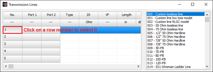
1. Select a row by clicking on the row number of your choice in the first column labeled ‘No.’, Fig. 2.

2. On the right-hand panel, choose a type of transmission line and double-click on your chosen type. The selected row will be automatically completed, Fig. 3.

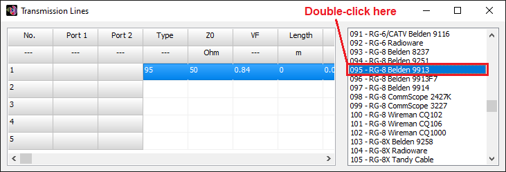
3. From type 3 onwards, the parameters correspond to real cable datasheets. If you wish to enter your own parameters, choose types 0, 1, or 2. To edit the value in a cell, double-click on the cell.

Note that in this procedure, the ports of the transmission lines have not been connected to the wire segments yet. This is explained in Connecting Transmission Lines.

The parameters that define a transmission line are:

1) Type: On the right-hand panel of the Transmission Lines window, there is a list of lines with the cable part number and the manufacturer in some cases. The first three types are used to input user-customized lines. The line type simply refers to its position in this list.

2) Z0: Nominal characteristic impedance, in Ohms. If a negative value is entered, the transmission line will be “crossed” with a 180° phase reversal with respect to the reference directions of the segments (the characteristic impedance of the line will of course be |Z0|).

3) VF: Velocity factor (dimensionless). The allowed range is 0 < VF <= 1.

4) Length: Length of the line, in the unit selected in the Preferences window (see Section “3.3 Preferences”). If a length of zero is entered, the length of the transmission line will be equal to the linear distance between the two wire segments connected at the ends of the line.

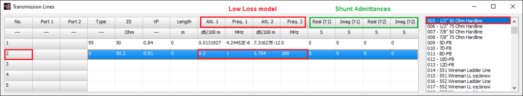
5) The K0, K1, K2, and K3 columns define the line losses for the so-called RLGC model. These four columns will change to Att. 1, Freq. 1, Att. 2, Freq. 2 when the chosen line model is that of low losses. These cells allow entering the attenuation curve of a real transmission line from its datasheet.

6) Real(Y1) and Imag(Y1) are the real and imaginary parts of the shunt admittance through Port 1 of the transmission line, in Siemens [S].

7) Real(Y2) and Imag(Y2) are the real and imaginary parts of the shunt admittance through Port 2 of the transmission line, in Siemens [S].

A transmission line without shunt admittances (Y1 = Y2 = 0) will always be symmetrical in the sense that if it is connected in reverse, i.e., by swapping ports 1 and 2, the same results will be obtained in a simulation. Ports 1 and 2 are identified so that the locations of the shunt admittances can be distinguished when they are not zero.

If you enlarge or maximize the Transmission Lines window, you will be able to see the columns corresponding to the loss model parameters and shunt admittances, Figs. 4 and 5. Initially, this window only displays cells up to the ‘Length’ column so that the user does not have to worry about the loss parameter values since these are automatically loaded when selecting a line type from the list. Adding an attenuation curve when modeling a cable that is not on the list is explained in Adding a Custom Lossy Line.