Design Guidelines for Skeleton Slot Antennas: A Simulation-Driven Approach

This article navigates the intricacies of Skeleton Slot antennas, exploring their sensitivity to geometric parameters and the transformative impact of a simulation-driven methodology. The Skeleton Slot is treated as an array of two loop antennas with a common feed point. We delve into the balance of loop perimeters, conductor radii, and aspect ratios, unraveling their influence on output parameters such as input impedance, VSWR, and gain. We present a script-driven approach to optimize designs, empowering engineers and enthusiasts to craft high-performance Skeleton Slot antennas. Bridging theory and application, the article showcases practical insights, making it an essential resource for anyone seeking to elevate their radio frequency design projects.

Introduction

Bill Sykes (call sign G2HCG) is acknowledged as the innovator behind the Skeleton Slot antenna, having successfully deployed it in VHF bands. The inherently versatile Skeleton Slot principle extends its utility to HF communication bands by scaling dimensions based on wavelength, with the physical antenna dimensions remaining practical within the 14-28 MHz bands. Noteworthy advantages of this design include its lightweight nature, ease of construction, low-angle radiation, bi-directional directivity, and the convenience of mounting it as a simple metal framework without the need for insulation.

The nomenclature “Skeleton Slot” is derived from the slot antenna concept. This aperture antenna is crafted by cutting a rectangular hole in a conducting sheet, essentially serving as a “photographic negative” of a dipole, where the slot functions as the radiating element. Reducing the metal sheet until it transforms into a rectangular wire frame results in the formation of the “skeleton slot.”

In our previous article, “A Closer Look at the HF Skeleton Slot Antenna,” we introduced a Skeleton model in AN-SOF and presented the results for the 15m (20 MHz) band. Expanding upon that analysis, this article delves into a comprehensive discussion of the skeleton slot from a general perspective, supported by the theory of loop antennas. This approach complements the insights provided by the inventor in the January 1955 issue of The Short Wave Magazine in the article titled “The Skeleton Slot Aerial System” (Vol. XII, No. 11, pp. 594-598). In that article, the author elucidates the antenna as an array of two closely positioned dipoles. Furthermore, we offer dimensioning guidelines for experimenters keen on venturing into antenna construction.

Geometry of Skeleton Slot and Loop Antennas

In Figure 1, a schematic representation of the Skeleton Slot antenna is presented, highlighting key dimensions:

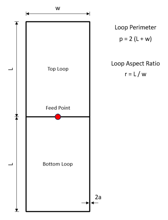
The skeleton slot, depicted in Figure 1, functions as a vertical antenna that can be conceptualized as an array comprising two identical, closely coupled loops—a top loop and a bottom loop. These loops share a common feed point located at the antenna’s center, where the feeding transmission line is connected.

In adherence to loop theory, when the loop contour spans approximately half a wavelength, it exhibits an input impedance transitioning from inductive to capacitive. This shift is characterized by high resistance and reactance values, indicative of a resonance akin to that observed in a parallel RLC circuit. Referencing the validation article “Input Impedance and Directivity of Large Circular Loops”, specifically Figure 2, illustrates the input impedance variation concerning the loop circumference measured in wavelengths, C/λ (see Figure 2 below). As the loop circumference approaches one wavelength, the capacitive (negative) reactance decreases in absolute value, reaching resonance similar to a series RLC circuit when the reactance approaches zero. Consequently, the resistance assumes manageable values in practice, approximately around 100 Ohms. The “useful zone” of the loop in practice is identified when C/λ ≈ 1, as shown in Figure 2.

While Figure 2 refers to circular loops, the analogous behavior is applicable to rectangular loops as well. Therefore, the practical utility of the loop is realized when its perimeter, denoted as ‘p,’ approaches one wavelength (p/λ ≈ 1).

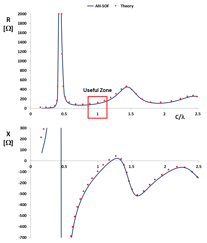
A further observation drawn from loops with circumferences comparable to the wavelength is the pronounced sensitivity of reactance to variations in the wire radius. This sensitivity manifests in a logarithmic manner, specifically proportional to ln(C/a), where ‘a’ denotes the wire radius.

Given its configuration, as previously mentioned, the Skeleton Slot antenna can be viewed as comprising two tightly coupled rectangular loops. Consequently, we can anticipate a behavior analogous to that described for loops in general.

Maintaining a constant loop aspect ratio (r = L/w) and conducting numerous calculations while varying the loop perimeter (p = 2(L + w)), we observe that the Skeleton Slot resonates when the loop perimeter is approximately one wavelength (p ≈ λ), aligning with expectations for a single loop. However, it’s crucial to note that this perimeter isn’t precisely equal to one wavelength; its value fluctuates based on the aspect ratio (L/w) and the wire radius compared to the loop perimeter (a/p). While the specific results of these calculations fall beyond the scope of this article, we will concentrate on the behavior of the skeleton slot when the perimeter of each loop approximates one wavelength. In this condition, the antenna approaches self-resonance, obviating the necessity for an impedance matching network at the feed point.

In Sykes’ article, the author employs the aspect ratio of the Skeleton Slot, expressed as 2L/w = 2r, rather than that of each individual loop. Through multiple measurements, the conditions for achieving a self-resonant antenna are outlined as follows:

1. An optimal aspect ratio of 3:1, i.e., 2r = 3, leading to r = 3/2 = 1.5 based on our definition.

2. The total length of the skeleton must be 2L = 0.56λ, so the loop length is L = 0.28λ.

3. The ratio of width to conductor diameter must be 32:1, denoted as w/(2a) = 32.

Given L = 0.28λ and r = L/w = 1.5, the resulting perimeter is calculated as p = 2 (0.28λ + 0.28λ/1.5) = 0.93λ. This closely aligns with our simulation calculations, indicating resonance when the loop perimeter approximates one wavelength. However, it’s essential to note that this resonance condition varies with the ratio of perimeter to conductor radius, denoted as p/a, rather than the ratio w/(2a). Subsequent results, presented in the following sections, illustrate that a thicker conductor necessitates an increased loop perimeter for the antenna to be self-resonant with a given aspect ratio. Conversely, a thinner conductor requires a decreased loop perimeter for the same resonant condition.

Script for Varying the Loop Aspect Ratio

A pivotal inquiry in Skeleton Slot antenna design revolves around determining the optimal aspect ratio. Is there a specific aspect ratio that outperforms others? This section aims to delve into this question, with the pursuit of an “optimal” point focusing on achieving a self-resonant antenna, thereby obviating the need for a matching network. In Sykes’ investigation, a conductor with a radius of 4.76mm (rounded up to 5mm in our study) was employed, corresponding to a 3/16″ radius (3/8″ diameter).

For our exploration, we maintain a fixed conductor radius of 5mm, and we ensure that the perimeter of each loop remains close to one wavelength, as previously discussed. Simulations conducted using AN-SOF are set at a frequency of 20 MHz (15-meter band). Importantly, the conclusions drawn from these simulations hold true for any frequency band, contingent upon scaling the antenna dimensions proportionally with the wavelength. Naturally, the resulting physical dimensions at a given frequency must be practical for constructing the antenna in practice.

To perform calculations with varying geometric parameters, we can leverage the “Run Bulk Simulation” function in AN-SOF in conjunction with a script in Scilab. For those unfamiliar with script programming, a comprehensive tutorial on antenna-related scripts is available in the article “Element Spacing Simulation Script for Yagi-Uda Antennas”, specifically focusing on Yagis with variable element spacing.

Description of Script Elements

Below, the script is provided to generate multiple files in .nec format, where the loop aspect ratio, L/w, is systematically altered while maintaining a fixed perimeter, p. Through multiple simulations, we have determined that the “optimal” p value, rendering the antenna self-resonant for a broad range of L/w ratios, is p = 14.8m at 20 MHz, corresponding to p = 0.99λ.

When the perimeter p is held constant and the loop aspect ratio is varied (r = L/w), the antenna dimensions can be calculated using the following formulas:

To expedite the task, consider creating a Skeleton Slot antenna model in AN-SOF or downloading the model provided in this article. Then, in AN-SOF, navigate to the File menu, select “Export Wires,” choose the file format “.sce,” and save the file. Subsequently, open the .sce file with Scilab and make the modifications as illustrated below:

// Script for AN-SOF Professional
// Skeleton Slot Antenna with varying aspect ratio

r_min = 1.0; // Min loop aspect ratio
r_max = 2.5; // Max loop aspect ratio
n = 20; // Number of intervals between r_min and r_max
f = 20.0; // Frequency in MHz
k = 0.987; // Factor for loop perimeter
p = k*299.8/f; // Loop perimeter [m] (299.8/f = wavelength at f MHz)
radius = 5; // Wire radius in [mm]
S = 11; // Number of segments per wire (it must be odd)

for i = 0:n, 
r = r_min + i*(r_max-r_min)/n; // Loop aspect ratio
w = 0.5*p/(r+1); // Loop width
L = r*w; // Loop length (total length of skeleton slot = 2L)

antenna = [ 
CM('Skeleton Slot Antenna')
CM('Loop length-to-width ratio = ' + string(r))
GW(1, S, 0, -0.5*w, 0, 0, 0.5*w, 0, radius*1e-3)
GW(2, S, 0, 0.5*w, -L, 0, -0.5*w, -L, radius*1e-3)
GW(3, S, 0, -0.5*w, L, 0, -0.5*w, 0, radius*1e-3)
GW(4, S, 0, 0.5*w, 0, 0, 0.5*w, L, radius*1e-3)
GW(5, S, 0, -0.5*w, -L, 0, -0.5*w, 0, radius*1e-3)
GW(6, S, 0, 0.5*w, 0, 0, 0.5*w, -L, radius*1e-3)
GW(7, S, 0, 0.5*w, L, 0, -0.5*w, L, radius*1e-3)
GE(0)
FR(0, 1, f, 0.0)
EX(0, 1, (S+1)/2, 1.4142136, 0)
EK()
];

mputl(antenna,'C:/AN-SOF/Skeleton_Ratio' + string(i) + '.nec');
end

This simple script streamlines the process, allowing for efficient exploration of the Skeleton Slot antenna’s behavior under varying loop aspect ratios. This script comprises two main elements:

1. Definition of Constants:

   – Fixed values for the extremes of the loop aspect ratio variation range.

   – Number of intervals ‘n’ to be calculated (with ‘n+1’ discrete points).

   – Loop perimeter ‘p’ and wire radius.

   – Numerically adjusted perimeter ‘p’ within 3 significant digits at p = 0.987λ.

2. ‘For’ Loop:

   – The script contains a “for” loop where the “antenna” matrix is defined. Each row contains commands (CM, GW, GE, FR, EX, EK) used to describe an antenna in NEC format.

   – Each generated .nec file (n+1 files) is named “Skeleton_Ratioi.nec” with i = 0, 1, 2, …, n.

This script is complemented by a second script that reads the results from CSV files and represents them graphically in plots. Additionally, there is a third script that contains the functions associated with NEC commands. To download these three scripts, click on the button provided above.

Running the Scripts in Combination with AN-SOF

Here are the steps to run this script, along with the one displaying graphs with results, in combination with AN-SOF:

1. Download the .zip file containing the three necessary scripts: NECcommands.sce, SkeletonSlot.sce, and SkeletonSlotResults.sce.

2. Unzip the file and save the scripts in a folder to run them from Scilab.

3. Start Scilab and open the scripts.

4. Run NECcommands.sce, which contains functions that write NEC commands.

5. Create a folder C:\AN-SOF and run SkeletonSlot.sce. The n+1 “.nec” files will be saved in this folder.

6. In AN-SOF, go to the menu Run > Run Bulk Simulation, navigate to the C:\AN-SOF folder, and select all the generated .nec files (you can press Ctrl + A). AN-SOF will calculate them one by one, saving the corresponding results in CSV files.

7. Return to Scilab and run the SkeletonSlotResults.sce script. Three graphs will be displayed: the gain, the input impedance, and the VSWR as a function of the loop aspect ratio.

With these scripts, you can obtain results that will be analyzed in the subsequent sections for the input impedance, VSWR, and antenna gain as a function of the loop aspect ratio.

Input Impedance, VSWR, and Gain vs. Aspect Ratio

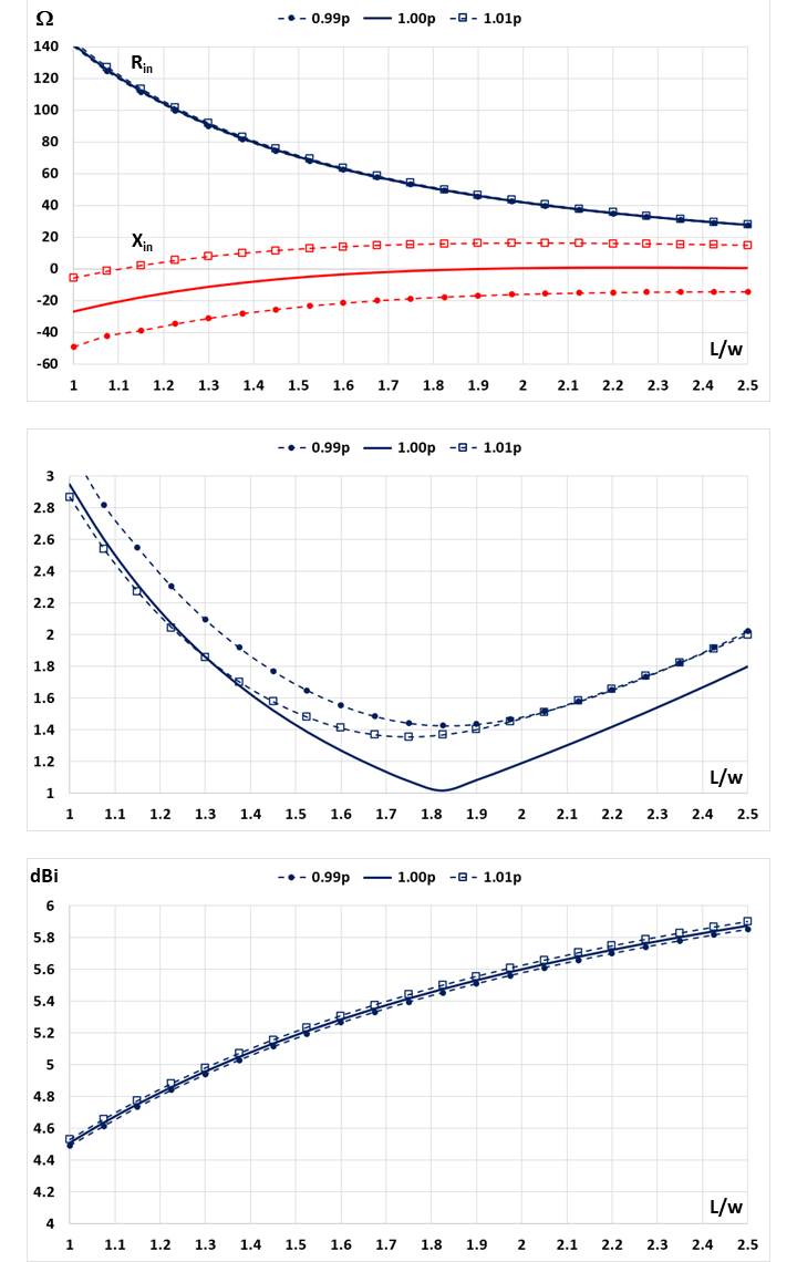
In Figure 3, the Skeleton Slot input impedance (R_in + jX_in) is depicted as a function of the loop aspect ratio, L/w. It’s crucial to note that the loop perimeter remains constant at approximately one wavelength, p ≈ λ, resulting in variable antenna length and width to uphold the constant perimeter. The relative sizes of the Skeleton Slot for three aspect ratios—L/w = 1, 1.8, and 2.5—are illustrated at the bottom of Figure 3. Note that, when L/w = 1, the loops form squares (L = w). These outcomes have been calculated for a conductor radius of 5mm.

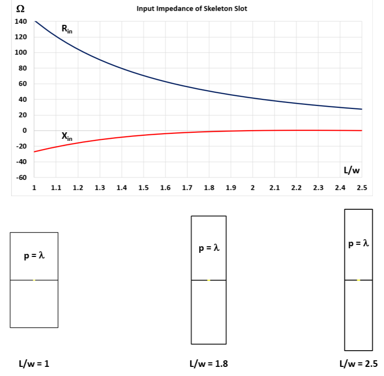
The input impedance unveils an intriguing property: commencing at an aspect ratio of 1.7, the antenna maintains self-resonance (X_in = 0) as the aspect ratio increases. The reactance curve (X_in) is notably flat with values that are practically manageable even when the loops form squares (L/w = 1). However, the input resistance, R_in, exhibits a more pronounced variation, initiating at 140 Ohms for L/w = 1 and steadily decreasing to approximately 30 Ohms for L/w = 2.5. The input impedance approaches 50 + j0 Ohms at L/w ≈ 1.8. This suggests an optimal point where the antenna achieves self-resonance without requiring an impedance matching network.

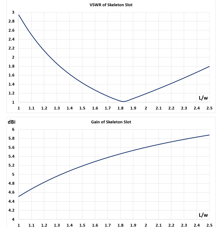
Within the range of L/w spanning from 1.6 to 2, we observe a practical sweet spot with the input resistance falling between 40 and 60 Ohms and the reactance approaching zero. Figure 4 (top) illustrates the Voltage Standing Wave Ratio (VSWR) as a function of the loop aspect ratio, considering a reference impedance of 50 Ohms. The “useful” range for VSWR falls within values of L/w between 1.6 and 2. Additionally, Figure 4 (bottom) showcases the gain of the skeleton slot, demonstrating a monotonic increase with the loop aspect ratio. Opting for L/w = 2 becomes advantageous if the design objective is to maximize gain.

In the subsequent sections, we will delve into an analysis of the skeleton slot’s sensitivity to variations in loop perimeter and conductor radius. This exploration will contribute to the establishment of simulation-driven design guidelines, enabling a more informed and optimized design process.

Sensitivity to the Loop Perimeter Around One Wavelength

With the established optimal loop perimeter for achieving a self-resonant antenna at p = 0.99λ, we explore the impact of a ±1% change in this perimeter. For a frequency of 20 MHz, corresponding to a wavelength of 15 meters, this adjustment would equate to a ±15 cm change in perimeter. Figure 5 (top) illustrates the input impedance as a function of the loop aspect ratio for three different perimeters: 0.99p, 1.00p, 1.01p, where p = 0.99λ.

Notably, the resistive part (R_in) demonstrates minimal variation with changes in perimeter, whereas the reactive part (X_in) undergoes a significant alteration. The sensitivity of the reactive part to changes in p is notably higher. An increase in perimeter results in an augmented reactance (X_in), while a decrease in perimeter leads to a diminished reactance. This observation suggests that the perimeter of the loops can serve as a tuning parameter for the antenna. If, for a given loop aspect ratio L/w, the antenna is not self-resonant (X_in ≠ 0), adjustments can be made by increasing the loop perimeter when X_in < 0 and decreasing it when X_in > 0. Consequently, the antenna can always be tuned to a self-resonant state, provided the ability to adjust its physical dimensions, manipulating both the loop perimeter and aspect ratio.

In the central part of Figure 5, the Voltage Standing Wave Ratio (VSWR) is presented as a function of the loop aspect ratio. The observed variation in VSWR is predominantly attributed to changes in reactance resulting from adjustments in the loop perimeter.

In our model, the antenna is considered in free space without the presence of a ground plane, and no resistivity has been added to the conductors, effectively eliminating power losses. This deliberate choice allows us to isolate the ideal behavior of the skeleton slot and analyze its parameters independently. In an antenna devoid of ohmic losses, the resistive component of its input impedance equals its “radiation resistance.” The gain of a lossless antenna is inversely proportional to the radiation resistance. If this resistance remains insensitive to changes in perimeter, we can anticipate a corresponding insensitivity in gain. This expectation is affirmed in Figure 5 (bottom), where the gain is depicted as a function of the loop aspect ratio for the three distinct values of loop perimeter used in the upper graphs.

Effect of Changing the Conductor Radius

The investigation explores the impact of changing the conductor radius on the input impedance, VSWR, and gain as a function of the loop aspect ratio. It is widely recognized that loops with a circumference close to one wavelength exhibit higher reactance for thinner wire radii. To quantify loop thickness, the loop perimeter to wire radius ratio, p/a, is commonly used. However, since the loop perimeter is held constant in our analysis, we solely vary the radius (a = 5mm) of the example model.

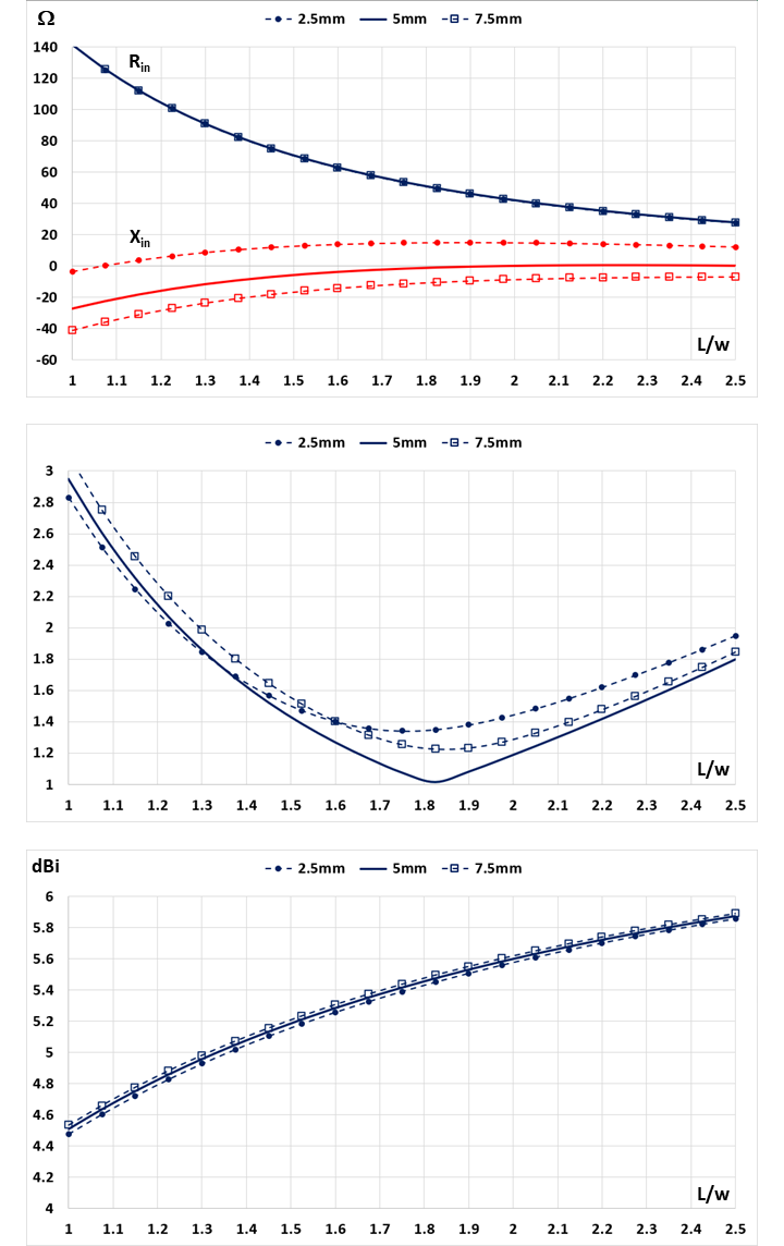
At the top of Figure 6, the input impedance of the Skeleton Slot is depicted as a function of the loop aspect ratio for three different conductor radii: a = 2.5mm, a = 5mm, a = 7.5mm. As observed, reactance increases with a thinner conductor and decreases with a thicker conductor. This observation, combined with insights from Figure 5 in the previous section, leads to the conclusion that the loop perimeter required for a self-resonant antenna is influenced by the wire radius. Given a specific loop wire thickness, p/a, the exact value of p for self-resonance depends on p/a itself, so we can write p(self-resonance) = k(p/a) λ, where k(p/a) is near 1. While it is not within the scope of this study to generate curves illustrating the behavior of the factor k(p/a), simulation tools like AN-SOF allow for a simulation-driven design, a topic to be discussed in the next section.

In the middle of Figure 6, the VSWR behavior is presented, with variations predominantly attributed to changes in input reactance. The bottom graph in Figure 6 illustrates the antenna gain, demonstrating no sensitivity to the wire radius, as expected, since the radiation resistance also remains insensitive to the wire radius, as indicated in the top graph of Figure 6.

Simulation-Driven Design of a Skeleton Slot Antenna

Having established the optimal relationships among the geometric parameters of the Skeleton Slot antenna, conceptualized as two closely coupled loops sharing a feeding point, we can now outline a procedural approach for designing such antennas using simulation tools like AN-SOF.

In practical scenarios, it’s common to have a conductor or wire with a specific diameter. Therefore, our initial step will involve setting the wire radius as a fixed parameter, followed by running simulations with slight variations in the perimeter of each loop, starting with p = λ as a reference. The previously described script can be employed for this purpose, keeping the perimeter constant while adjusting the loop aspect ratio.

Following this, the subsequent step is to identify the loop aspect ratio that maximizes gain within an acceptable VSWR range. To illustrate this procedure, we will present example calculations for HF and VHF, namely for operating frequencies of 14 MHz and 145 MHz, respectively.

HF Skeleton Slot Antenna

We will take as a reference the same example presented in Sykes’ article in “The Short Wave Magazine.” For applications in the HF band, at an operating frequency of 14 MHz, in accordance with the Sykes criterion (loop width to conductor diameter of 32:1), a 4¾-inch wire would be required—an impractical dimension. The author suggests using multiple wires (e.g., 6) to form a circular contour with the desired diameter. However, in our demonstration, we aim to show that achieving a self-resonant antenna with a 3/8″ diameter conductor is indeed feasible.

Figure 7 illustrates the results for input impedance and VSWR obtained from the script with the following input parameters:

f = 14.0; // Frequency in MHz
k = 0.987; // Factor for loop perimeter
p = k*299.8/f; // Loop perimeter [m] (299.8/f = wavelength at f MHz)
radius = (3/16)*25.4; // Wire radius in [mm]
S = 7; // Number of segments per wire (it must be odd)

The gain is not displayed since it closely resembles the previously shown results. Figure 7 illustrates that the optimal loop perimeter is maintained with a factor k = 0.987, ensuring the antenna is self-resonant at 14 MHz. The chosen design point is L/w = 1.825, precisely where the VSWR exhibits a dip. Following this, we open the corresponding AN-SOF file (Skeleton_Ratio11.emm) and perform a frequency sweep around the central frequency of 14 MHz.

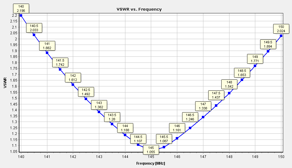
Figure 8 portrays the VSWR as a function of frequency for the Skeleton Slot with L/w = 1.825. The observation indicates an achieved bandwidth of almost 600 KHz (for VSWR < 2), equivalent to 4.3% in the 14 MHz band. The gain obtained is 5.5 dBi.

If we were to choose L/w = 2.05 and conduct a frequency sweep, we would notice a reduced bandwidth of 500 KHz, signifying that making the skeleton slot slimmer is no longer advantageous, despite yielding slightly higher gain.

VHF Skeleton Slot Antenna

For the operation of the Skeleton Slot at 145 MHz, we maintain the same conductor diameter of 3/8″ (wire radius, a = 3/16″). In this case, by executing the script with the same perimeter factor as the one used before (k = 0.987, with the loop perimeter being p = kλ), we obtain a negative input reactance. As we learned in the previous sections, we will then need to lengthen the loop perimeter to increase the reactance and approach resonance.

Through several calculations (not shown here), we determined that the optimal value is k = 1.03, for which the results are shown in Figure 9. Therefore, a loop perimeter that is 3% longer than a wavelength is necessary in this case to obtain a self-resonant antenna in a wide range of loop aspect ratios. The chosen design point is L/w = 1.9.

f = 145.0; // Frequency in MHz
k = 1.03; // Factor for loop perimeter
p = k*299.8/f; // Loop perimeter [m] (299.8/f = wavelength at f MHz)
radius = (3/16)*25.4; // Wire radius in [mm]
S = 7; // Number of segments per wire (it must be odd)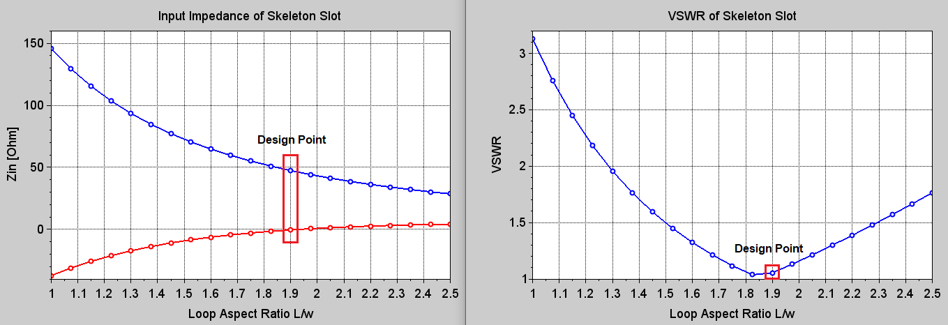

By opening the file corresponding to this aspect ratio (Skeleton_Ratio12.emm for L/w = 1.9) with AN-SOF and performing a frequency sweep around 145 MHz, we obtain the VSWR curve shown in Figure 10. In this case, the obtained bandwidth is 9.5 MHz (for VSWR < 2), which represents 6.6% with respect to the center frequency of 145 MHz. The gain obtained is 5.7 dBi.

With this last example, we believe we have covered the design of Skeleton Slot antennas in a depth that perhaps has not been done before. We complete the information for the designer with a few words about the number of segments, set using the “S” variable in the script. Since each loop has a perimeter of one wavelength, the total number of segments used per wavelength is 4S. Through comparisons with theoretical data for the loops, we have established that about 30 or 40 segments per wavelength are sufficient to reproduce theoretical data. Note that when S = 11 in the Skeleton Slot example for 20 MHz, we have 44 segments per λ, while with S = 7, we have 28 segments per λ. If you have measured data at hand, it is advisable that the number of segments be increased until the simulation model reproduces these experimental data.

Conclusions

In this comprehensive article, we conducted an in-depth study of the Skeleton Slot antenna, emphasizing its applicability across frequency bands by normalizing dimensions to the wavelength. While the theoretical analysis holds true for any frequency, practical construction considerations will be constrained by physical dimensions and installation space available in a specific frequency band.

The Skeleton Slot antenna, conceptualized as an array of two loops with a common feed point, was meticulously examined. We provided a script enabling the alteration of the antenna’s aspect ratio, generating multiple files for bulk simulation in AN-SOF. This facilitated the extraction of input impedance, VSWR, and gain as functions of the aspect ratio. The results highlighted the antenna’s self-resonance when the perimeter of each loop is approximately one wavelength.

We explored how the antenna’s behavior changes with variations in loop perimeter and conductor thickness. The optimal design point for the Skeleton Slot was identified as the loop aspect ratio minimizing VSWR for a given conductor radius. The simulation-driven design methodology can be summarized in the following steps:

1. Choose the conductor diameter for constructing the Skeleton Slot.

2. Define the operating frequency and determine the optimal perimeter using the provided scripts. The self-resonance loop perimeter is typically around one wavelength.

3. Choose the design point by selecting the loop aspect ratio that minimizes VSWR (or maximizes gain, depending on the objective). Conduct a frequency sweep to ascertain the obtained bandwidth.

This simulation-driven design approach is particularly valuable for amateur radio enthusiasts, antenna hobbyists, or RF professionals embarking on projects involving Skeleton Slot antennas. We trust that this article will serve as a valuable resource for those interested in exploring and implementing Skeleton Slot antenna designs.

---