Plotting 3D Far-Field Patterns

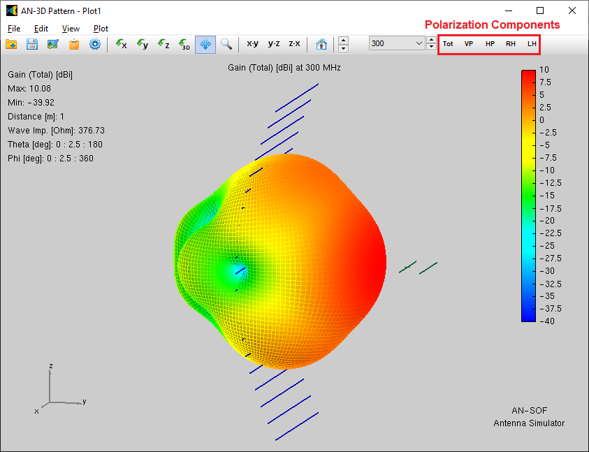
The far-field distribution can be visualized as a comprehensive 3D plot by selecting Results > Plot Far-Field Pattern > 3D Plot from the AN-SOF main menu. This command launches the AN-3D Pattern application, which renders the radiation pattern in a three-dimensional space, using a dynamic color scale to represent field intensities across the lobes.

Field Metrics and Polarization Decomposition

The Plot menu within AN-3D Pattern provides access to a wide array of electromagnetic metrics (Fig. 1), including:

• Power Density and E-field
• Directivity and Gain: Available in both numerical (linear) and dBi scales.
• Radiation Pattern: Normalized to unity (1.0) or 0 dB.
• Axial Ratio: Presented as a dimensionless value or in dB.

Each metric can be decomposed into its constituent polarization components using the toolbar buttons (Tot, VP, HP, RH, LH). This allows for the isolated analysis of:

• Linear Polarizations: $\theta$ (Theta, Vertical) and $\phi$ (Phi, Horizontal).
• Circular Polarizations: Right-Handed (RHCP) and Left-Handed (LHCP).

Radar Cross Section (RCS)

For simulations involving plane wave excitation (such as scattering analysis or an antenna in receiving mode), the software enables the plotting of the Radar Cross Section (RCS). The resulting 3D visualization represents the scattered field pattern as observed in the far-field region, where field amplitude decays by $1/r$ and power density by $1/r^2$.

Analyzing the Axial Ratio

The 3D Axial Ratio pattern illustrates the ratio between the minor and major axes of the polarization ellipse.

• Linear Polarization: Indicated by a value of 0.
• Circular Polarization: Indicated by a value of 1.

While the 3D plot excels at showing the magnitude of the axial ratio, the sign (which defines the sense of rotation as RHCP or LHCP) is best verified in a 2D rectangular plot. However, the rapid-switching polarization buttons on the 3D toolbar, RH and LH, provide an efficient alternative for identifying dominant polarization handedness.

Navigation and Dynamic Frequency Sweeping

The 3D environment is fully interactive, allowing for detailed inspection of the radiation structure:

• Manipulation: Use the 3D Rotation or Move buttons on the toolbar to rotate or translate the view by clicking and dragging. Zooming is handled via the mouse wheel.
• Dynamic Frequency Sweep: A key feature of the AN-3D Pattern toolbar is the ability to toggle the operating frequency. By using the up-down arrow buttons next to the frequency display, users can observe the radiation lobes evolve dynamically, effectively creating an animation of the antenna’s wideband performance.

3D Visualization and Data Management in AN-3D Pattern

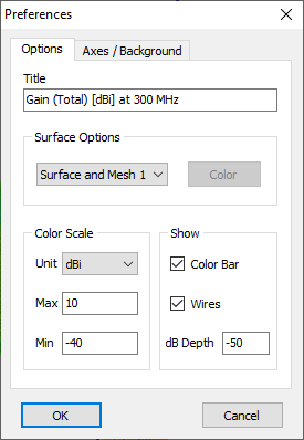
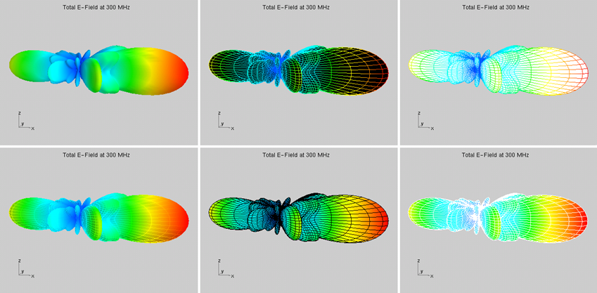
To access the Preferences dialog box in the AN-3D Pattern application, navigate to Edit > Preferences in the main menu (Fig. 2). This interface allows for deep customization of the 3D visualization, including the appearance of the colored surface and the density of the mesh overlay on the radiation lobes (Fig. 3).

For enhanced spatial context, you can superimpose the physical wire structure onto the radiation pattern by checking the Wires option within the “Show” panel. This panel also provides controls for the graph’s scale and the toggle for displaying the coordinate axes ($x, y, z$).

Data Export and Tabulation

While the 3D graphical representation is intended for visualization, the raw far-field data for a specific frequency can be extracted by returning to the AN-SOF main menu. Select Results > List Far-Field Pattern to generate a tabular view of the results. From there, click the Export button to save the dataset as a CSV (Comma Separated Values) file, which can be imported into external spreadsheet or analysis software.

Note

• If discrete sources were used as the excitation of the structure, the plotted far-field represents the total field.
• If an incident plane wave was used as the excitation, the plotted far-field represents the scattered field.