Modeling a Circular Loop Antenna in AN-SOF: A Step-by-Step Guide

This step-by-step guide empowers you to simulate circular loop antennas in AN-SOF. We’ll configure the software, define loop geometry, and explore how its size relative to wavelength affects radiation patterns and input resistance. Gain valuable insights into this fundamental antenna type!

This article provides a step-by-step guide to modeling a circular loop antenna using AN-SOF software. Circular loops are a common antenna type, and their analysis requires curved segments within the simulation environment. The guide will detail the configuration process, including defining the loop geometry, setting up the frequency sweep, incorporating a voltage source, and analyzing the key parameters like radiation pattern and input resistance. This guide is valuable for RF engineers, ham radio enthusiasts, students, and antenna design professionals seeking to utilize AN-SOF for circular loop antenna simulations.

1. Specifying the Simulation Setup

This section outlines the initial setup steps required to model a circular loop antenna in AN-SOF. We’ll configure a frequency sweep to analyze the antenna’s behavior across a specified range.

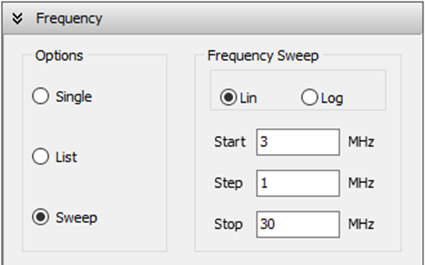
Frequency Sweep:

1. Navigate to the Setup tab and select Sweep within the Frequency panel.
2. Choose Lin for a linear frequency sweep. This allows for evenly spaced data points across the desired range.
3. Define the sweep parameters:
   • Start frequency: 3 MHz
   • Step: 1 MHz (adjust as needed based on desired resolution)
   • Stop frequency: 30 MHz

These settings establish a linear sweep from 3 MHz to 30 MHz with 1 MHz increments between each data point (as shown in Fig. 1).

Additional Settings:

• Environment: Ensure that None is selected in the Ground Plane box within the Environment panel. This removes any ground plane influence from the simulation, which might not be relevant for a free-space loop antenna.
• Excitation: In the Excitation panel, verify that Discrete Sources is selected. This indicates that we’ll define a lumped source (voltage or current) to excite the antenna later in the modeling process.

By following these steps, we’ve established the foundation for our loop antenna simulation by configuring the frequency sweep and essential simulation settings in AN-SOF. The next section will delve into defining the geometry of the circular loop itself.

2. Defining the Circular Loop Geometry

This section focuses on creating the circular loop geometry within the AN-SOF workspace:

1. Access the Draw Menu: Navigate to the Workspace tab. Right-click on an empty area within the workspace and select Circle from the pop-up menu.
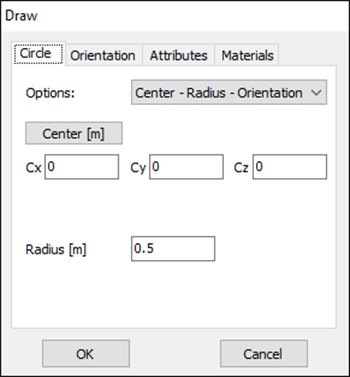
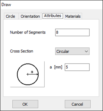
2. Specify Loop Parameters: The Draw dialog box for the circle will appear (Fig. 2). Define the following parameters for your loop antenna using the provided tabs:
   • Center: (Cx, Cy, Cz) = (0, 0, 0) (Circle tab)
   • Radius: 0.5 meters (Circle tab)
   • Segments: 8 (Attributes tab)
   • Cross-section type: Circular (Attributes tab)
   • Cross-section radius: 5 millimeters (Attributes tab)

Segment Selection: The number of segments used to discretize the loop circumference is crucial for accurate simulation results. While 8 segments are a reasonable starting point, a convergence study might be necessary to ensure sufficient accuracy, especially for electrically large loops. As a rule of thumb, aim for 10-20 segments per wavelength at the highest frequency of interest.

Electrical Size Considerations: It’s important to consider the loop’s electrical size relative to the wavelength. At 30 MHz (the highest frequency in your sweep), the wavelength (λ) is indeed 10 meters, and the loop’s circumference (0.314λ) is close to one-third of a wavelength. This suggests the loop might not be electrically small at the high end of the frequency range. This characteristic will affect the antenna input impedance and radiation pattern.

Assigning the Excitation Source:

1. Right-click on the circular loop within the AN-SOF workspace.
2. From the pop-up menu, select Source/Load.
3. Choose to add a voltage source and position it at the first segment of the loop.

For detailed instructions on source placement and parameter definition, refer to the AN-SOF documentation’s ‘Adding Sources‘ section.

3. Running the Simulation and Analyzing Results

This section guides you through initiating the simulation process and analyzing the obtained results in AN-SOF:

1. Run Simulation: Locate the Run Currents and Far-Field (F11) button on the toolbar and click it. This initiates the simulation, calculating the current distribution on the loop and its far-field radiation pattern across the defined frequency sweep.
2. Visualizing the Radiation Pattern: Once the simulation is complete, click the Far-Field 3D Plot button on the toolbar. This will display the radiation pattern of the loop antenna in a 3D format (AN-3D Pattern application similar to Fig. 3).
3. Frequency-Dependent Analysis: The AN-3D Pattern toolbar offers functionalities to explore the radiation pattern’s behavior at different frequencies within the sweep range.
   • Frequency selection dropdown menu: This menu allows you to directly choose a specific frequency point to view its corresponding radiation pattern.
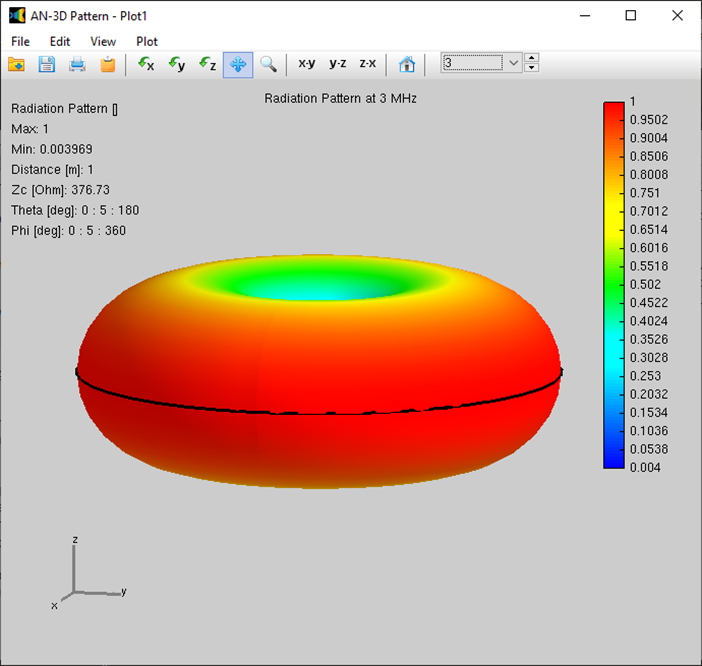
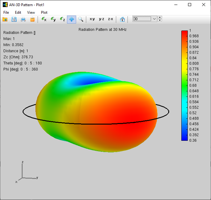
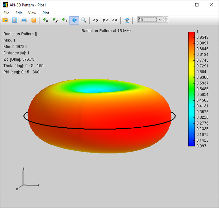
   • Frequency navigation buttons: Utilize the up and down arrow buttons on the toolbar to navigate through the calculated frequencies and observe the dynamic changes in the radiation pattern. As expected for a circular loop antenna, the pattern should exhibit a doughnut-like shape at lower frequencies.
4. Input Resistance Analysis: Navigate to the Results tab within AN-SOF. Here, you should observe a very low input resistance value, likely around 0.000195 Ohm at 3 MHz.
5. Comparison with Theoretical Radiation Resistance: The well-known formula for the radiation resistance, R_r, of an electrically small loop antenna is R_r = 31,200 (A/λ²)². Applying this formula with the loop’s area (A) and the wavelength (λ) at 3 MHz, you obtain a theoretical value of R_r ≈ 0.000192 Ohm. The close agreement between the simulated and theoretical values at 3 MHz demonstrates that the loop behaves according to the small loop antenna model at lower frequencies within the sweep range.

Important Note:

It’s important to remember that the formula used for radiation resistance applies to electrically small loops. As mentioned earlier, the chosen loop dimensions might not be electrically small across the entire frequency sweep (especially at 30 MHz). This will lead to deviations between the theoretical and simulated results at higher frequencies.

Figure 3 illustrates the frequency dependence of the loop antenna’s 3D radiation pattern. Subfigures (a), (b), and (c) depict the patterns at 3 MHz, 15 MHz, and 30 MHz, respectively.

By following these steps, you’ve successfully run the simulation, analyzed the radiation pattern, and compared the input resistance with theoretical expectations.