Evaluating EMF Compliance – Part 1: A Guide to Far-Field RF Exposure Assessments

Ensuring Electromagnetic Field (EMF) compliance is crucial for safeguarding individuals and the environment from potential adverse effects of radiofrequency (RF) exposure. This article provides a comprehensive guide to EMF compliance assessment using far-field RF exposure evaluations.

The article delves into the concepts of antenna radiation, the near-far field boundary, and Effective Isotropic Radiated Power (EIRP) compliance thresholds. It also provides a practical step-by-step approach to EIRP-based EMF compliance assessment using AN-SOF Antenna Simulation Software. This approach is demonstrated for antenna configurations with and without ground planes, considering the impact of feed lines on EIRP values.

Key takeaways from this article include:

✅ EMF compliance assessment is essential for ensuring RF exposure safety.

✅ EIRP is a crucial parameter in EMF compliance assessment.

✅ Antenna configuration and feed lines influence EIRP values.

✅ The near-far field boundary determines the appropriate methodology for EMF compliance calculations.

✅ AN-SOF can be used to model antenna configurations and perform accurate EIRP calculations.

Understanding the Framework of RF Exposure Regulations

In March 2020, the International Commission on Non-Ionizing Radiation Protection (ICNIRP) published its new guidelines, ICNIRP 2020, on limiting exposure to radio frequency (RF) electromagnetic fields (EMF) in the frequency range of 100 kHz to 300 GHz. Most countries worldwide currently have regulations on RF-EMF exposure and set limits based on the previous ICNIRP 1998 guidelines and are expected to update their regulations in accordance with the revised limits, published in 2020. A summary of the main differences between ICNIRP 2020 and previous guidelines can be found in ICNIRP 2020c.

The US Federal Communications Commission (FCC) has followed its own path by publishing RF exposure limits since 1996, before the ICNIRP 1998 guidelines were published (see OET Bulletin 65 Edition 97-01). While in other countries, such as the UK, the ICNIRP guidelines are followed. Ofcom follows the 1998 edition of these guidelines in the UK. All of these regulations are based on studies and research on the potential for non-ionizing radiation to damage the human body.

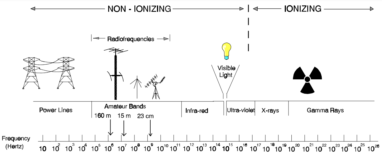
In the frequency bands up to 300 GHz, the main effect of electromagnetic waves is to heat biological tissues by exciting the molecules, which causes an increase in temperature. Unlike ionizing radiation such as X-rays, which can cause electrons to jump to higher energy levels, changing the state of atoms and potentially causing DNA damage. Figure 1, extracted from FCC Bulletin 65 Edition 97-01, illustrates the electromagnetic spectrum, where we can see that RF signals used for telecommunications, including the amateur radio bands, are well below the UV and X-rays frequencies.

One figure used to evaluate the heating of tissues is the Specific Absorption Rate (SAR), which is a measure of the rate at which RF energy is absorbed per unit mass of tissue. Based on SAR studies of canonical antennas operating in close proximity to the human body and numerical models of these antennas, the communications regulators set maximum reference limits for the electric field, magnetic field, and power density to reduce exposure to RF EMFs.

Every transmitting antenna or radiating system must comply with the RF EMF exposure limits set by the regulators in each country or region. Exposure limits to non-ionizing radiation are set well below the minimum levels required to cause adverse health effects in humans associated with RF-induced heating in the body. The ICNIRP guidelines, adopted in most countries, are independent of the technology used to transmit the RF waves and apply equally to all mobile and fixed installation antenna technologies within the specified frequency range.

This article focuses mainly on EMF compliance in amateur radio bands, but the same principles can be applied to other parts of the frequency spectrum and other types of activities. Although each country or region establishes its own criteria, there is a lot of similarity between regulations around the world. Therefore, we will use as examples the guidelines published by the FCC in the US and by Ofcom in the UK. In particular, the amateur radio societies in each country or region, the American Radio Relay League (ARRL) and the Radio Society of Great Britain (RSGB), respectively, have published online calculators in the form of web apps (see ARRL calculator and RSGB calculator) that allow estimating parameters to establish whether a station complies with the respective regulations.

In reality, compliance should be established by performing precise EMF measurements in the vicinity of each station and for each set of parameters, or equipment configuration as Ofcom conveniently calls it, which includes frequency, RF power, transmission mode, transmission/reception times, antenna type, antenna height, and installation site. Carrying out these measurements would be impractical and extremely onerous for most radio amateurs or licensees, since they require specialized and calibrated instruments that are usually expensive. Therefore, the regulatory bodies have taken a pragmatic approach and accept that assessments be carried out based on the online calculators that they themselves have published.

In the UK, it is mandatory for licensees to keep a record of these assessments to be presented in case of receiving an inspection. While in the US, it is not mandatory but it is suggested to keep these records to be presented in cases of third-party complaints. These online calculators are based on closed-form formulas that are valid for the far-field region of antennas, which can be convenient as a first approximation. However, it is advisable to resort to much more accurate antenna modeling and simulation software tools available today, in order to have a more realistic picture of the compliance of a station or “equipment configuration.”

The fact of setting EMF threshold levels implies that we can determine a compliance boundary or exclusion zone around an antenna from which the radiated field takes levels below the maximum thresholds provided by the regulators. Exclusion zones, therefore, are areas where access to the general public should be restricted. Regarding the marking of these areas and the measures that the people responsible for the installation must take to prevent access by the general public who may be exposed to RF levels dangerous to health, we recommend consulting the regulations of each country. In the first instance, if the exclusion zone cannot be controlled, actions should be taken such as lowering the RF power of the transmitter, reducing the duty cycle, elevating, redirecting, or relocating the antenna.

The existence of an exclusion zone around an antenna implies that we must consider the different EMF regions. In radio amateur activities, operators are normally familiar with RF communication at long distances from the antenna, in the so-called far-field region. However, near the antenna, the EMF levels are often very high, so the exclusion zones are usually in the near-field region of antennas. Due to this differentiation, we have divided this article into two parts. This first part deals with how to calculate the EMF compliance in the far-field region, while the second part will deal with how to perform the calculations in the near-field region of antennas. For these reasons, the next section deals with the EMF regions around an antenna.

Antenna Radiation and the Near-Far Field Boundary: Essential Concepts

Establishing a definitive boundary between the near- and far-field regions of an antenna poses a significant challenge in RF engineering. This stems from the intricate distribution of electromagnetic fields in the vicinity of the antenna, lacking a clear demarcation between the two regions.

In the immediate vicinity of the antenna, electric field lines originate and terminate on the antenna’s metallic components, dispersing themselves into the surrounding space in a complex manner. In this region, electrical energy is stored, oscillating in cycles dictated by the operating frequency. Similar behavior is observed for the magnetic field, with its lines forming closed loops. Both fields exchange energy during each cycle, mimicking the operation of an LC oscillator.

The balance of electrical and magnetic energy may not always be equal, resulting in a non-zero net energy. This imbalance manifests as either an inductive (positive) reactance at the antenna terminals when magnetic energy prevails or a capacitive (negative) reactance when electrical energy dominates. This region near the antenna, where the distributed LC oscillator exists in the surrounding space as field lines coupled to the antenna structure, is termed the near-field region.

While Figure 2 depicts the near-field region as an LC oscillator enclosed within a spherical boundary around an antenna, it’s important to note that this boundary may not always conform to a spherical shape.

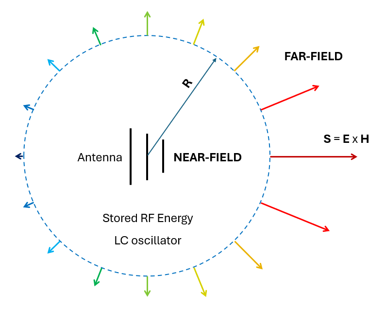
Beyond the oscillation of stored electric and magnetic RF energies within the near-field region, there exists a flow of radiant energy that escapes from this oscillator to the antenna’s exterior. This energy flux is characterized by the Poynting vector (S = E x H), or power flux density, measured in Watts per square meter of the wavefront, where E represents the electric field and H represents the magnetic field. As we gradually move away from the antenna, the near-field region transitions into the far-field region, where the field lines have completely detached from the antenna and evolved into an electromagnetic wave that propagates radially outward.

The flux of radiant power to the antenna’s exterior manifests as a resistance at the antenna terminals, termed radiation resistance. Measured in Ohms, radiation resistance does not represent power losses (ohmic losses) due to heat dissipation; rather, it represents the radiated power from the antenna. In essence, we have an RLC oscillator distributed in the space surrounding the antenna, continuously pumping radiant energy out of the antenna.

Inevitably, ohmic losses occur in the metallic components of the antenna and its surrounding environment, including soil conductivity, insulating materials, and support structures. Consequently, the input power to the antenna, injected into the antenna terminals by a transmission line, for example, is divided into radiated power and lost power. In a transmitting antenna, the goal is to maximize radiated power, thereby maximizing the antenna’s efficiency, ensuring that most of each supplied Watt is transformed into radiated power.

It is often possible to distinguish a transition region between the near- and far-field regions, sometimes called the radiative near-field region. In the far-field region, the propagating wave has a spherical wavefront, and on the surface of this sphere, the electric (E-field) and magnetic (H-field) fields are perpendicular to each other, perpendicular to the power density vector (S), and oscillate in phase. Moreover, they maintain a fixed relationship, E/H ≈ 377 Ω, the so-called free-space characteristic impedance. This is a TEM (transverse electromagnetic) wave, where the fields are transverse to the direction of propagation. Far away from the antenna, an observer will perceive a small portion of the spherical wavefront, which is usually approximated by a plane wave, and from there comes the TEM plane wave approximation.

Figure 2 depicts the power density S [W/m²] on a spherical wavefront of radius R centered at the antenna. The power density points radially outwards and is not generally uniform on the wavefront, but exhibits directionality.

In most textbooks, we will find the following boundaries between field regions:

• For electrically large antennas, whose maximum dimension D is much greater than the wavelength (D >> λ), the far-field region begins at a distance that depends on the size of the antenna: R = 2D²/λ.

• For electrically small antennas, whose maximum dimension D is much smaller than the wavelength (D << λ), the far-field region begins at a distance independent of the antenna size: R = λ/(2π).

In practice, these limits tend to be overly conservative, necessitating more sophisticated methods when a more precise delineation of the near-far field boundary is required with a specified tolerance. One such method is described in the article Wave Matching Coefficient: Defining the Practical Near-Far Field Boundary. This approach utilizes the concept of wave impedance and defines a coefficient analogous to return loss in transmission lines to determine the near-far field boundary based on a tolerance in decibels. The resulting inter-region boundary is irregularly shaped around the antenna and requires extensive post-processing of the calculated results, but it is the most accurate method for determining the near-far field boundary.

In part 2 of this article, we will present a simpler method based on computing the near E and H fields of an antenna on a sphere centered on the geometric center of the antenna and comparing the field values to reference levels published by regulatory bodies.

This first part focuses on the far-field region, where regulators typically recommend using the concept of Effective Isotropic Radiated Power (EIRP) to determine if a configuration complies with EMF safety standards. EIRP allows for easy assessment of compliance when it remains below the established maximum levels. Most low-power transmitting stations meet these limits and thus do not require the determination of exclusion zones or exposure distances through near-field calculations. However, for configurations exceeding the EIRP maximums, calculating the electric field, magnetic field, and power density is essential to determine the exclusion zone by ensuring that their values stay below the recommended reference levels.

While a station may be considered EMF compliant based on EIRP levels, if calculations indicate an exclusion zone within a few centimeters of the antenna’s metallic parts, regulators often recommend establishing a minimum safety zone of a couple of meters from the antenna. For instance, in the UK, a minimum safety distance of 2.4 meters (8 ft) is mandated regardless of exclusion zone calculations.

In mobile applications, where antennas are typically positioned close to the human body, the FCC in the US has established a different exposure analysis method based on Specific Absorption Rate (SAR). This method is mandatory for all radios with antennas that are within 20 cm of a person.

EIRP: Definition, Calculation, and Exposure Thresholds

The area of a sphere with radius “R” is given by 4πR². Let’s consider a radial distance R from the geometric center of the antenna of interest, as depicted in Figure 2. As we increase the radius of the sphere, moving away from the antenna, the radiated power density “S” in Watts per square meter (W/m²) over the sphere decreases proportionally to the inverse of the square of the distance (1/R²). This inverse relationship holds true when the distance R is significantly greater than the size of the antenna (D) and the wavelength (λ), indicating that we are in the far-field region (R >> D and R >> λ).

The radiated power density, S, is not uniformly distributed over the sphere of radius R (see Figure 2). While some antennas radiate omnidirectionally along circles obtained by slicing the spherical wavefront, there’s always a direction where the power density drops to zero due to the cancellation of the vector E and H fields. Consequently, there’s no such thing as an isotropic radiator, where the power density is perfectly uniform in all directions in 3D space, at all points of the spherical wavefront. Instead, the power density exhibits a directional pattern over the wavefront.

Since the power density, S, is measured in W/m², multiplying each square meter of the sphere by the “average” value of S in that portion of the surface gives us the power in Watts that radiates through that square meter of the wavefront. To determine the total radiated power, P_r, we repeat this procedure over the entire surface of the wavefront and sum up the partial radiated powers. Once we have the total radiated power, P_r [W], we can calculate an average power density, S_av [W/m²], simply by dividing P_r by the area of the sphere, 4πR². Therefore:

Conversely, if we calculate S_av by averaging S over the surface of the sphere, we get the radiated power, P_r, as:

Imagine replacing the antenna with an ideal isotropic radiator that emits a perfectly uniform power density over the entire sphere’s surface, in all directions, that is exactly equal to S_av, the average power density radiated by the original antenna. In this scenario, the isotropic radiator would radiate power effectively as P_r = 4πR²S_av. This magnitude is known as the Average Effective Isotropic Radiated Power (EIRP_av), which essentially represents the total power radiated outwards by the antenna. Consequently, we have:

It’s important to note that this is a “spatial average,” not a “time average.” Although an isotropic radiator is a theoretical concept, it serves as an ideal reference point. Those who find the isotropic radiator concept challenging can instead use a half-wave dipole as the reference radiator, as we will discuss later.

As mentioned, the radiated power emitted by the antenna outwards is a portion of the input power at the antenna terminals supplied by the transmitter. The remaining portion is lost as heat dissipation. The radiated power is the one we want to maximize. To transmit a wave carrying energy effectively, we must maximize the energy supplied by the transmitter, allowing it to propagate over great distances and facilitate communication. Telecommunications (“tele” means distant or far away in Greek) is the ultimate goal of our passion for antennas!

Note that the radiated power density decreases with the square of the distance (1/R² law), while the area of the spherical wavefront increases with the square of the distance (4πR²). By multiplying this area by S_av, these effects cancel out, and the radiated power remains independent of the distance to the antenna. This is an expected outcome, as the total radiated power, total losses, and total input power at a given frequency must always remain constant. This adherence to the principle of energy conservation can be summarized as: Input Power = Radiated Power + Lost Power.

The EIRP in equation (3) represents the spatially averaged EIRP, calculated using the spatially averaged power density, S_av. Since antennas exhibit directionality (as evidenced by the nonexistence of an isotropic radiator), for setting exposure thresholds, it is crucial to consider the peak power density (worst case) rather than the average. Therefore, we can define the peak EIRP in terms of the peak power density, S_Peak (maximum value on the wavefront), as follows:

Hereafter, we will omit the “Peak” subscript in the EIRP, implying that we are referring to the maximum EIRP, which serves as the basis for regulatory exposure limits.

Returning to the spherical wavefront with radius R and area 4πR², centered on the geometric center of the antenna (technically, the “phase center” would be more precise, but we won’t delve into that here), the peak gain of the antenna, G, is defined as:

Where P_i represents the input power in Watts. The gain is a far-field parameter that, similar to the radiated power in equation (3), is independent of distance. Instead of establishing a maximum exposure limit for the peak power density, S_Peak, regulatory bodies publish maximum thresholds for the EIRP. The peak EIRP is a parameter that is only well-defined in the far-field region, where it becomes distance-independent due to the inverse square law governing the decrease of peak power density S_Peak with distance. Combining equations (4) and (5), it is straightforward to demonstrate that:

In other words, the EIRP can be determined by multiplying the antenna gain G (numerical gain, not in dBi) by the power supplied to the antenna terminals, P_i, in Watts.

The definition of antenna gain in equation (5) corresponds to the gain relative to an isotropic radiator. When using a half-wave dipole as a reference antenna, which has a numerical gain of 1.64 (2.15 dBi), the Effective Radiated Power (ERP) is defined as:

Expressing the powers in dBW (decibels with respect to 1 W), we have the following equivalent expressions for the ERP in dBW:

For low-power transmitting stations, regulatory bodies often provide exemption EIRP or ERP thresholds. The limits that determine whether a station is exempt from regular evaluations vary by country. Generally, the powers involved are extremely low, resulting in fields with levels far below the thresholds considered hazardous. The ICNIRP 1998 and 2020 guidelines do not address EIRP or set limits for it; they only focus on SAR, electric field, magnetic field, and power density values. Assessing compliance based on EIRP is a practical and relatively straightforward approach to determine whether a station or equipment configuration adheres to EMF safety standards.

In 1997, the FCC published a table of power thresholds in OET Bulletin 65, Edition 1997, for the routine evaluation of amateur radio stations. This table directly provided limits for the transmitter power or PEP (Peak Envelop Power) input to the antenna, P_i. Exemption from performing routine ERP-based assessments was only applicable for repeater stations. The FCC referred to the ERP instead of EIRP, and the table is reproduced below in Table 1.

Band	Wavelength	Evaluation Required if Power (Watts) Exceeds:
MF	160 m	500
HF	80 m	500
	75 m	500
	40 m	500
	30 m	425
	20 m	225
	17 m	125
	15 m	100
	12 m	75
	10 m	50
VHF	All bands	50
UHF	70 cm	70
	33 cm	150
	23 cm	200
	13 cm	250
SHF	All bands	250
EHF	All bands	250
Repeater Stations	All bands	non-building-mounted antennas: height above ground level to lowest point of antenna < 10m and power > 500W ERP building-mounted antennas: power > 500W ERP

In 2021, updated FCC rules affected amateur radio stations previously exempted by the old rules. As described in the QST Magazine (September 2021, pages 60-62) article “Understanding the Changes to the FCC RF Exposure Rules” by Ed Hare (W1RFI), this update included an FCC table providing ERP thresholds depending on frequency and observation distance. This table, replicated in Table 2 below, allows us to determine if a station is exempt.

Transmitter Frequency [MHz]	Threshold ERP [W]
0.3 – 1.34	1,920 R2
1.34 – 30	3,450 (R/f)2
30 – 300	3.83 R2
300 – 1,500	0.0128 R2 f
1,500 – 100,000	19.2 R2

The exemption is granted simply because the calculation yields ERP values below the thresholds. Performing this calculation is already an assessment in itself, which determines that the station is EMF compliant. For the exception in Table 2 to apply, the separation distance R in meters must be at least λ/(2π). Note that this is the theoretical distance for the near-far field boundary applicable to electrically short antennas.

For more in-depth information on RF exposure and amateur radio stations, we highly recommend the book by Ed Hare (W1RFI) “RF Exposure and You,” published by the ARRL, 1998-2003.

In contrast to the FCC’s approach, Ofcom in the UK simplifies the matter by establishing that a transmitting station is low power compliant when the peak EIRP is ≤ 100 W and the averaged-in-time EIRP is ≤ 10 W, for any frequency range. This approach introduces the concept of time averages, which play a crucial role in assessing RF exposure risks.

The Significance of Time Averages

The duration of exposure to an RF signal significantly impacts its biological effects. Exposure to the same radiated power for 1 minute is not equivalent to exposure for 1 hour. When the exposure time is short, the human body’s tissues can dissipate the excess heat, minimizing potential harm. As a result, the average power supplied by the transmitter over time is the critical factor.

The average power of a transmitter, typically a fraction of its peak power, is significantly influenced by the duty cycle, also known as the duty factor, of its transmit mode. This factor represents the percentage of time the transmitter actively sends a signal compared to the total time period. Notably, the duty cycle varies depending on the modulation technique employed. Table 3 provides an overview of the typical duty cycles for various transmit modes. The mode factor represents the multiplier applied to the transmitter’s Peak Envelope Power (PEP) to obtain the average input power, which ultimately contributes to the EIRP calculations.

Transmit Mode	Mode Factor	Duty Cycle	dB
AFSK	1.0	100%	0.0
AM	0.3	30%	-5.2
Analog TV	0.6	60%	-2.2
Carrier	1.0	100%	0.0
CW (Morse code)	0.4	40%	-4.0
DMR 1 slot	0.46	46%	-3.4
DMR both slots	0.92	92%	-0.4
Dstar	1.0	100%	0.0
FM	1.0	100%	0.0
FSK	1.0	100%	0.0
FSK441	1.0	100%	0.0
FT4	0.34	34%	-4.7
FT8	0.42	42%	-3.8
JT65	0.39	39%	-4.1
JT9	0.41	41%	-3.9
MSK144	1.0	100%	0.0
Other Digital	1.0	100%	0.0
Other WSJT sub-modes	0.4	40%	-4.0
PSK31/PSK63	0.75	75%	-1.2
RTTY	1.0	100%	0.0
SSB	0.2	20%	-7.0
SSB Processed	0.5	50%	-3.0
System Fusion	1.0	100%	0.0
WSPR	0.92	92%	-0.4

Furthermore, it’s crucial to consider the percentage of time the station remains active within a specific time frame, such as a 6-minute period. As an example, if telegraph mode transmits for only 3 minutes out of every 6 minutes, the power level considered for the EIRP calculation undergoes a 50% reduction. Therefore, to determine the average input power, we need to multiply the PEP by both the mode factor and the fraction of time within each 6-minute block that the transmitter is active.

Compliance Assessments for Non-Exempt Stations

For stations that do not meet the exemption criteria (FCC) or the low power compliance criteria (Ofcom), a more rigorous assessment is required. Electric field, magnetic field, and power density must be calculated using near-field formulas to establish precise exclusion zones. These near-field values are then compared with the established maximum reference levels to determine whether the station is EMF compliant.

Near-field closed form mathematical expressions are often highly complex and are only available for simple canonical antennas, such as electrically short dipoles or small loops. This complexity necessitates the use of antenna simulation software like AN-SOF.

The assessment of RF exposure from amateur radio stations involves various considerations, including power thresholds, time averages, and near-field calculations. Understanding these factors is crucial for ensuring the safe operation of amateur radio equipment and minimizing potential health risks.

EIRP-Based EMF Compliance Assessment: A Simulation-Driven Approach

With the knowledge of the antenna’s numerical gain, G, and the input power, P_i, supplied by the transmitter, the EIRP can be easily obtained by multiplying both quantities, as demonstrated in equation (6). Both the online calculators provided by the ARRL and the RSGB include antenna gain as an input parameter. These calculators also offer a list of standard antennas with known gains, which are theoretical values.

The impact of antenna height on a lossy ground plane on the gain is only considered approximately, as the soil conductivity and dielectric constant cannot be entered (an average reflection coefficient is used in online calculators). Additionally, the effect of supports or obstacles that may exist in the antenna’s vicinity is neglected. In such cases, antenna simulation software like AN-SOF can be employed to obtain a more accurate calculation of the gain and, consequently, the EIRP. Notably, AN-SOF directly provides the peak EIRP as a function of frequency in the results table called Power Budget, from which a plot of EIRP vs. frequency can be generated.

As an example, we present far-field simulations for a 17m band Delta Loop Beam antenna, where we utilize the EIRP to establish EMF compliance in the far-field region. As mentioned earlier, if a station or equipment configuration fails to meet the EIRP test, exclusion distances must be determined based on near-field calculations, which will be covered in part 2 of this article.

Delta Loop Beam Analysis in Free Space

The 17m Band 2-Element Delta Loop Beam, a straightforward design we’ll examine in this article, represents the simplest two-element array that can be constructed using delta loops to achieve a directional antenna. The analysis focuses on the 17m band, encompassing frequencies from 18.068 to 18.168 MHz.

This antenna array naturally resonates near the band center, exhibiting an input impedance of approximately 50 Ohms, eliminating the need for an impedance matching network. For this model, the antenna is assumed to be operating in free space, without a ground plane. Initially, we’ll evaluate EMF compliance under these ideal conditions. Subsequently, we’ll introduce a ground plane, raise the antenna to a specific height, and incorporate a lossy coaxial cable as the antenna feed line to assess the impact on EIRP.

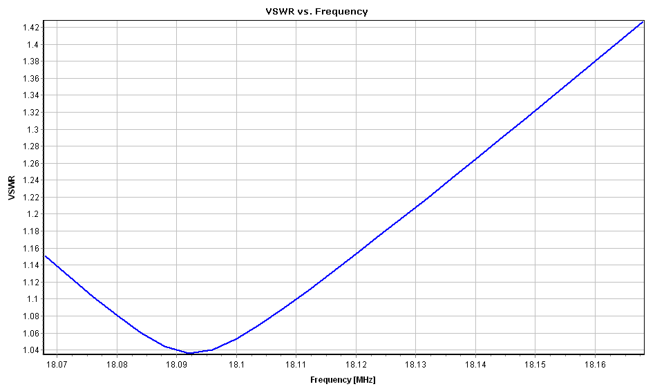
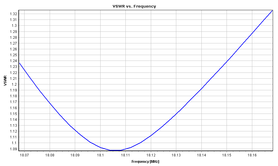
Figure 3 depicts the Voltage Standing Wave Ratio (VSWR) as a function of frequency for the Delta Loop Beam in free space. The antenna resonates at 18.096 MHz, displaying an impedance of 52 – j0.15 Ohms (VSWR = 1.04) at this frequency. To set the input power at the antenna terminals, navigate to the Setup tab > Excitation panel, select “Set Input Power,” and enter the power in Watts. Entering 10 W and then proceeding to the main menu > Results > Power Budget generates the table shown in Figure 4.

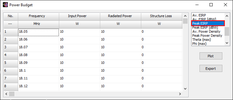
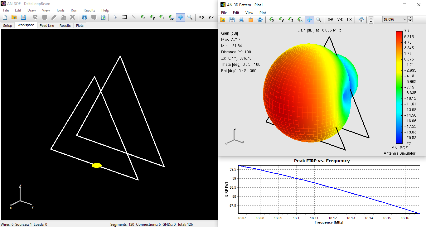
To visualize the EIRP, locate the Peak EIRP option in the right-hand panel of the Power Budget window. Double-clicking on this option generates a plot of EIRP in Watts as a function of frequency. Similarly, double-clicking on “Peak EIRP [dBW]” displays the EIRP in decibels with respect to 1 W. Figure 5 presents the results, including the antenna model in the AN-SOF workspace, the 3D radiation pattern representing the gain in dBi at 18.096 MHz, and the EIRP in Watts as a function of frequency. The peak gain is 7.7 dBi. The EIRP attains 59 W at the resonant frequency and peaks at 59.7 W within the operating bandwidth. The model can be downloaded by clicking the button below Figure 5.

In accordance with Table 1 above (1997 FCC rules), the maximum allowable input power to the antenna for the 17m band is 125 W, exempting the station from conducting an assessment. The set input power of 10 W falls well below this threshold. However, following the 2020 FCC update, referring to Table 2, we determine the ERP threshold for maximum allowable exposure as ERP = 3,450(R/f)² for frequencies within the range 1.34 – 30 MHz. In this case, f = 18.096 MHz, and considering the minimum acceptable distance, R = λ/(2π) = 299.8/18.096/6.28 = 2.64 m. Substituting these values for f and R yields an ERP threshold of ERP = 3,450 x (2.64/18.096)² = 73.4 W. According to equation (7), we have EIRP = 1.64 x 73.4 = 120 W. At the minimum allowable distance of 2.64 m, our 59 W EIRP antenna delivers an EIRP value that is almost half of the threshold for maximum permitted RF exposure. Therefore, our configuration complies with FCC EMF criteria.

Under Ofcom’s criteria, the permissible peak EIRP is 100 W, which our antenna configuration adheres to. However, Ofcom also mandates that the time-averaged EIRP be limited to 10 W. In this example, if we transmit continuously (100% of the time) using a transmit mode that provides the antenna with the full 10 W of transmitter PEP, we exceed the time-averaged EIRP threshold.

To reduce the average EIRP from 59 W to 10 W, we need to adjust the input power by a factor of 10/59 ≈ 0.17. With a duty cycle of 100% (mode factor = 1), this implies that we could transmit only 1 minute out of every 6-minute block (1/6 ≈ 0.17). Failure to meet this condition necessitates the establishment of an exclusion zone, which will be discussed in part 2 of this article.

Ofcom guidelines stipulate that the safety distance should be at least 2.4 m (8 ft) in all circumstances. Interestingly, this closely aligns with the 2.64 m minimum distance calculated based on the FCC’s R = λ/(2π) formula. As mentioned in the previous section, this theoretical boundary demarcates the near-field and far-field regions for electrically short antennas.

Delta Loop Beam Raised Above a Ground Plane

To assess the impact of the ground plane, we elevate the Delta Loop Beam to a height of 10 meters. Since the base of each delta already has a Z = 10m coordinate in the AN-SOF model, we only need to enable the real ground plane, which is positioned at Z = 0 by default. Navigate to the Setup tab > Environment and select the “Real” option under “Ground Plane”. Choose “Sommerfeld-Wait/Asymptotic” and “Moderate” for the soil parameters, resulting in a conductivity of 0.003 S/m and a permittivity (dielectric constant) of 4. Run the simulation by clicking the Run Currents and Far-Field (F11) button on the toolbar.

Figure 6 depicts the VSWR, indicating a slight shift in the resonant frequency to 18.116 MHz, where the input impedance is 55 – j0.3 Ohm (VSWR = 1.1).

While the effect of the ground plane is subtle in the VSWR curve, it becomes significantly evident in the radiation pattern shown in Figure 7, where the peak gain reaches 12 dBi.

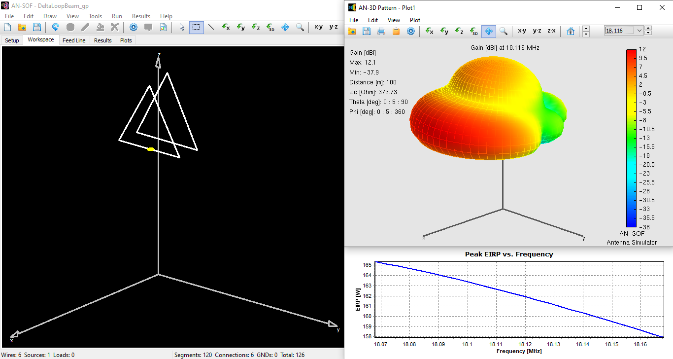
This substantial gain increase translates into a dramatic change in EIRP, as illustrated in the lower right plot of Figure 7. At the resonant frequency, the EIRP is 162 W, and within the operating frequency range, it peaks at 165 W. Applying the 2020 FCC rules, this value exceeds the maximum permitted RF exposure of 120 W calculated in Table 2 at the minimum distance of R = 2.64m. However, the antenna is now positioned 10m above ground. Assuming a safety margin of 2m above ground, which exceeds the height of an average person potentially walking under the antenna, we can set a radial distance R = 8m and recalculate the EIRP threshold. This calculation yields EIRP = 1.64 x 3,450 x (8/18.116)² = 1,103 W. With an EIRP of 162 W, we fall well below this threshold, demonstrating that the station complies with FCC EMF criteria.

FCC criteria are based on a separation distance R from the antenna to establish an EIRP threshold for a given frequency (Table 2). This corresponds to a far-field calculation, where a compliance boundary is determined by the radial distance R. In contrast, under Ofcom criteria, since we exceed the 100 W peak EIRP threshold, we must determine the exclusion zone by performing near-field calculations and comparing them to the permitted reference levels. This distinction between FCC and Ofcom criteria highlights the importance of understanding the regulatory framework applicable to amateur radio station operations. Both sets of guidelines aim to ensure that RF exposure levels remain within safe limits and protect individuals from potential harm.

Impact of the Feed Line

To incorporate the effect of the transmission line connecting to the antenna terminals, navigate to the Feed Line tab in AN-SOF. Here, select the cable type and its associated parameters. For this example, we’ll use a Belden 8267 RG-213 cable, which has a nominal characteristic impedance of 50 Ohms and a velocity factor of 0.66. AN-SOF automatically sets these line parameters along with the attenuation curve, determined by the parameters K0 (DC losses), K1 (skin effect), and K2 (dielectric losses). Next, specify the center frequency of 18.116 MHz. AN-SOF will automatically connect the corresponding antenna input impedance at one end of the transmission line, eliminating the need for manual input impedance entry. Figure 8 illustrates the Feed Line tab with the completed setup.

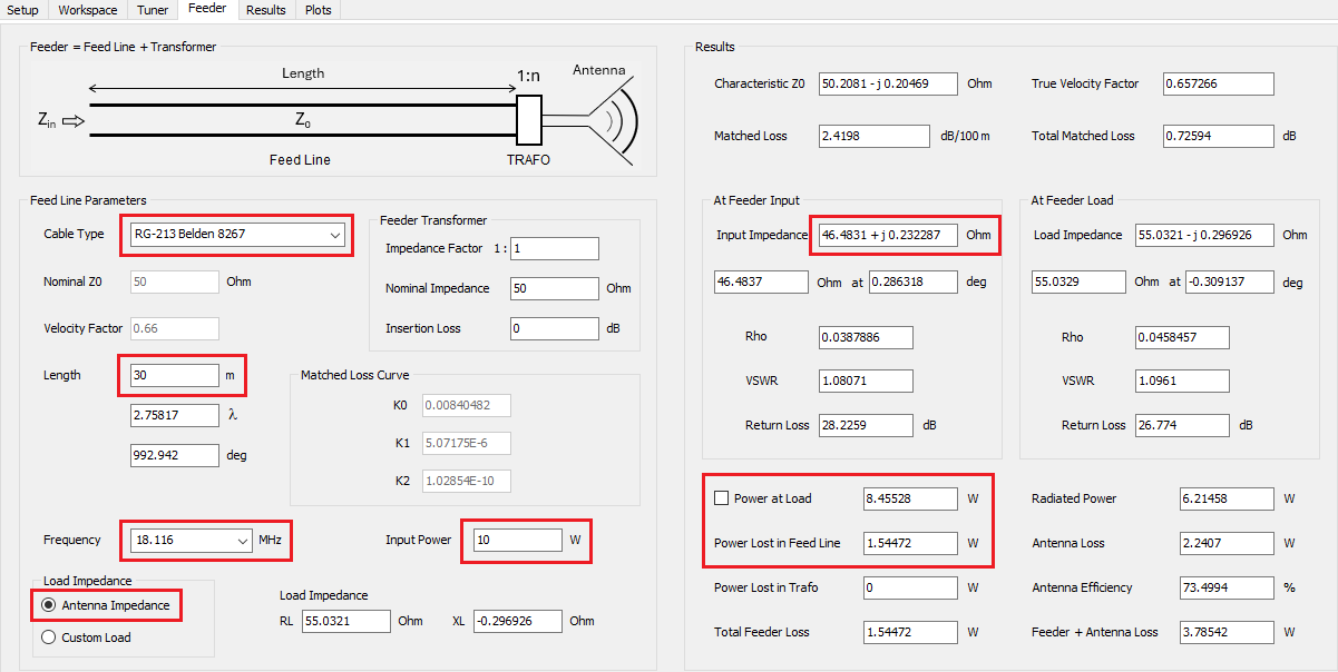
Enter an input power of 10 W and a transmission line length of 30 m (remember that the antenna is 10 m high). The “Results” panel on the right side of the “Feed Line” tab automatically updates the results as the input parameters on the left side are modified. The “Results” panel provides various details, including the impedance at the line input, which is the end connected to the transmitter supplying 10 W. At the bottom, we find the Power at Load/Antenna, which is 8.46 W (rounded to 3 digits), while the Power Lost in Line is 1.54 W. As expected, the sum of both powers, the power supplied to the antenna and the power lost on the feed line, equals the 10 W provided to the line.

To update the EIRP values, return to the Setup tab > Excitation panel and enter the reduced input power of 8.46 W. Then, proceed to the main menu > Results > Power Budget and replot the peak EIRP vs. frequency. At the center frequency, due to feed line losses, the EIRP has decreased by 25 W, from 162 W to 137 W. Figure 9 compares the antenna model with and without the feed line.

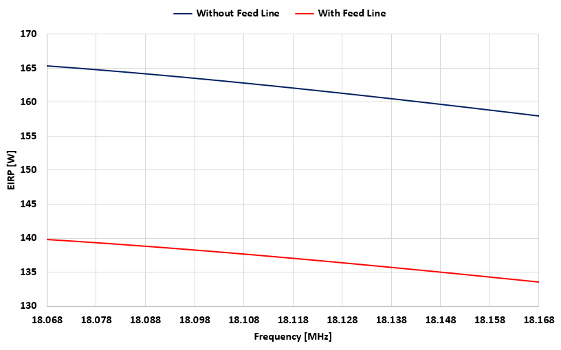
This example highlights how feed line losses can reduce EIRP and potentially bring a configuration into compliance with EMF regulations.

Conclusions

This article has provided a comprehensive overview of electromagnetic field (EMF) compliance assessment using far-field RF exposure evaluations. The focus has been on understanding the framework of RF exposure regulations, antenna radiation and the near-far field boundary, EIRP calculation and exposure thresholds, and the significance of time averages. Additionally, the article has presented a step-by-step approach to EIRP-based EMF compliance assessment using simulation tools, considering cases with and without ground planes and the impact of feed lines.

Key takeaways from this article include:

• EMF compliance assessment is crucial for ensuring the safety of individuals and the environment from potential harmful effects of RF exposure.

• RF exposure regulations provide limits on EIRP, the Effective Isotropic Radiated Power, to control exposure levels.

• The near-far field boundary determines the appropriate methodology for EMF compliance calculations.

• Far-field assessment involves calculating EIRP at a specified distance from the antenna and comparing it to regulatory thresholds.

• Simulation tools like AN-SOF can be used to model antenna configurations and perform accurate EIRP calculations.

• Factors like ground planes and feed lines can influence antenna performance and EIRP values.

The first part of this two-article series has focused on far-field RF exposure assessments. The second part will delve into near-field assessments and exclusion zone calculations, providing a complete understanding of EMF compliance evaluation techniques.

Disclaimer

Golden Engineering Ltd., developer of the AN-SOF Antenna Simulation Software, strives to provide accurate and reliable software for antenna modeling and simulation. However, the company assumes no responsibility for the consequences of using the software or the results obtained from its use. It is the sole responsibility of the software user or the person performing the calculations to ensure the accuracy and validity of the results. AN-SOF has been developed with the utmost diligence, incorporating numerical calculation methods aligned with the current state of the art in Computational Electromagnetics. Furthermore, the AN-SOF Knowledge Base provides numerous articles that validate the software’s calculations against theoretical and experimental results.

Despite these efforts, errors may occur due to user input, misinterpretations of results, or other factors beyond the control of Golden Engineering Ltd. These errors could lead to incorrect EIRP values or inaccurate electromagnetic field assessments, potentially exposing individuals to impermissible levels of RF signals. Therefore, Golden Engineering Ltd. explicitly disclaims any and all liability for any harm, injury, or damage resulting from the use of the AN-SOF Antenna Simulation Software or the interpretation of its results. The software user or the person performing the calculations assumes full responsibility for the accuracy and validity of the results and their implications for public safety.

---