1.4 The Hertzian Dipole – FREE SAMPLE

Heinrich Hertz and the Hertz Potential

Heinrich Rudolf Hertz (1857–1894) was a German physicist whose pioneering experiments provided the first direct evidence of electromagnetic waves, as predicted by James Clerk Maxwell’s equations. In 1887, Hertz generated and detected radio waves in the laboratory, demonstrating that they exhibited the same properties of reflection, refraction, polarization, and interference as light waves. His work not only confirmed Maxwell’s electromagnetic theory but also laid the foundation for the development of wireless communication and antenna theory. In recognition of his contributions, the unit of frequency, the hertz (Hz), was named in his honor.

In the early formulations of electromagnetic radiation problems, a mathematical tool known as the Hertz potential was often employed. This approach represented the fields in terms of an auxiliary vector potential from which the electric and magnetic fields could be derived. While historically important and still useful in certain contexts, the Hertz potential has largely been superseded by the now standard representation of the electromagnetic field in terms of a scalar potential $V$ and a vector potential $\mathbf{A}$.

The study of the Hertzian dipole, an idealized antenna consisting of a very short current element, is named in tribute to Heinrich Hertz. Despite its simplicity, this model plays a central role in antenna theory: it is not only the conceptual building block of more complex antennas, but also the starting point for deriving general expressions of radiated fields in free space.

Field Representation by Scalar and Vector Potentials

In what follows, we will need a result derived directly from Maxwell’s equations, known as the Continuity Equation. Starting with Ampère’s law in phasor form (1.1.33) for time-harmonic fields, if we apply the divergence operator and recall that the divergence of a curl is zero, $\nabla \cdot (\nabla \times \mathbf{H}) = 0$, we obtain

$\displaystyle \nabla \cdot \mathbf{J}(\mathbf{r}) \,+\, j \omega \varepsilon \, \nabla \cdot \mathbf{E}(\mathbf{r}) \,=\, 0 \qquad (1)$

Substituting Gauss’s law for electricity (1.1.34) into (1) leads us to the continuity equation in the frequency domain:

$\displaystyle \nabla \cdot \mathbf{J}(\mathbf{r}) \,=\, -j \omega \, \rho(\mathbf{r}) \qquad (2)$

If instead we start with Maxwell’s equations in the time domain, it is straightforward to obtain the general form of the continuity equation:

$\displaystyle \nabla \cdot \mathbf{J}(\mathbf{r}, t) \,=\, – \, \frac{\partial \rho(\mathbf{r}, t)}{\partial t} \qquad (3)$

This equation expresses the law of conservation of electric charge: the rate of decrease of charge density ($\partial \rho / \partial t$) within a given volume equals the negative divergence of the current density ($\nabla \cdot \mathbf{J}$), which represents the net current flowing out of that volume. In essence, charge is neither created nor destroyed, it simply moves.

Finally, in the limit of zero frequency, $\omega \to 0$, Eq. (2) reduces to $\nabla \cdot \mathbf{J} = 0$, from which Kirchhoff’s current law for lumped circuits can be directly derived.

At DC (direct current) regime, since $\omega \to 0$, Faraday’s law implies that the electric field is irrotational, i.e., a conservative field, which can be expressed as the gradient of an auxiliary scalar potential function $V$:

$\displaystyle \nabla \times \mathbf{E} = \mathbf{0} \;\; \implies \;\; \mathbf{E} = -\nabla V \quad \text{for } \; \omega \to 0$

The minus sign is a historical convention. We can verify it by recalling that the potential difference between two points $\mathbf{a}$ and $\mathbf{b}$ is given by integrating the conservative electric field $\mathbf{E}$ along any path connecting them. Since the field is conservative, the integral is path-independent and depends only on the potentials at the endpoints, $V(\mathbf{a})$ and $V(\mathbf{b})$:

$\displaystyle – \int_{\mathbf{a}}^{\mathbf{b}} \mathbf{E} \,\cdot\, d\mathbf{l} \,=\, \int_{\mathbf{a}}^{\mathbf{b}} \nabla V \,\cdot\, d\mathbf{l} \,=\, V(\mathbf{b}) \,-\, V(\mathbf{a})$

Here, $d\mathbf{l}$ represents an infinitesimal vector element tangent to the chosen integration path. From this, Kirchhoff’s voltage law follows naturally: the sum of all voltage drops around any closed loop in a circuit equals zero.

However, in the general case $\omega \neq 0$, and especially at high frequencies, the electric field is not conservative ($\nabla \times \mathbf{E} \neq \mathbf{0}$). This indicates that a term is missing from the static formulation, a term that does depend on the integration path. To uncover it, recall Gauss’s law for magnetism (1.1.35), which states that the magnetic field is divergence-free,

$\nabla \cdot \mathbf{H} = 0$,

making it a solenoidal field. Consequently, it can always be written as the curl of an auxiliary magnetic vector potential $\mathbf{A}$:

$\displaystyle \mathbf{H} \,=\, \frac{1}{\mu} \, \nabla \times \mathbf{A} \qquad (4)$

The factor $1/\mu$ is a conventional choice, historically used in this formulation. Equation (4) holds at all frequencies, including $\omega = 0$.

Substituting (4) into Faraday’s law (1.1.32) yields

$\displaystyle \nabla \times \mathbf{E} \,=\, -j \omega \, \nabla \times \mathbf{A} \qquad (5)$

Equation (5) reveals the missing term. Since the curl of a gradient is always zero, $\nabla \times (\nabla V) = \mathbf{0}$, the most general form of the electric field valid at any frequency can be written as

$\displaystyle \mathbf{E} \,=\, -\, j \omega \mathbf{A} \,-\, \nabla V \qquad (6)$

Equations (4) and (6) are fully consistent with Maxwell’s equations, and it is straightforward to verify that the $\mathbf{E}$ and $\mathbf{H}$ fields expressed in this way satisfy them. It is important to emphasize that $\mathbf{A}$ and $V$ are auxiliary potentials, not uniquely defined: adding a constant to either leaves the fields unchanged.

The advantage of this representation is that it provides a systematic way to derive solutions of Maxwell’s equations in the presence of free sources: charge density $\rho$ and current density $\mathbf{J}$. Moreover, these solutions are remarkably general and form the foundation for analyzing and calculating antenna behavior.

Let us now derive the wave equations for the scalar and vector potentials. Since time-harmonic electric and magnetic fields satisfy the homogeneous Helmholtz equations (1.1.36) and (1.1.37) in free space, or in a LIH medium without free sources, thus giving rise to electromagnetic waves, it is reasonable to expect that $V$ and $\mathbf{A}$ must also behave as scalar and vector waves, respectively.

Substituting (4) and (6) into Ampère’s law (1.1.33), and recalling that for any vector field

$\displaystyle \nabla \times (\nabla \times \mathbf{A}) \,=\, \nabla (\nabla \cdot \mathbf{A}) \,-\, \nabla^2 \mathbf{A}$,

together with $k^2 = \omega^2 \mu \varepsilon$, and then rearranging terms, we obtain:

$\displaystyle \nabla^2 \mathbf{A} \,+\, k^2 \mathbf{A} \,=\, \nabla \!\left(\nabla \cdot \mathbf{A} \,+\, j \omega \mu \varepsilon \, V\right) \,-\, \mu \, \mathbf{J} \qquad (7)$

Since we seek an expression for $\mathbf{A}$ that depends only on the current density $\mathbf{J}$, we can force the term in parentheses in (7) to vanish by choosing

$\displaystyle V \,=\, \frac{j}{\omega \mu \varepsilon} \, \nabla \cdot \mathbf{A} \qquad (8)$

This condition is known as the Lorenz gauge. As previously noted, we have some freedom in defining $V$ and $\mathbf{A}$: not only can constant fields be added, but different choices of “gauge” are also possible. It is straightforward to verify that adopting the Lorenz gauge (8) does not alter the field expressions obtained from Maxwell’s equations. With this choice, (7) reduces to the inhomogeneous Helmholtz equation for the vector potential:

$\displaystyle \nabla^2 \mathbf{A} \,+\, k^2 \mathbf{A} \,=\, – \mu \, \mathbf{J} \qquad (9)$

Applying the divergence operator to (6), using Gauss’s law for electricity (1.1.34), and substituting the Lorenz gauge (8), we obtain the inhomogeneous Helmholtz equation for the scalar potential:

$\displaystyle \nabla^2 V \,+\, k^2 V \,=\, – \,\frac{\rho}{\varepsilon} \qquad (10)$

We have thus confirmed our initial assumption: $V$ and $\mathbf{A}$ satisfy wave equations and can indeed be regarded as scalar and vector waves, respectively.

When we studied the isotropic point source in Section 1.2, we showed that exciting the Helmholtz equation with a Dirac delta function $\delta(\mathbf{r})$ at the origin yields the Green’s function given by (1.2.11), where the distance $r$ is measured from the position of the isotropic point source.

To generalize, suppose the source is located at an arbitrary point $\mathbf{r}’$ and the observation point is at $\mathbf{r}$. The distance between source and observation points is then $|\mathbf{r} – \mathbf{r}’|$, and the Green’s function in free space or in a LIH medium becomes

$\displaystyle G(\mathbf{r}, \mathbf{r}’) \,=\, \frac{e^{-jk \, |\mathbf{r} \,-\, \mathbf{r}’|}}{4\pi \, |\mathbf{r} \,-\, \mathbf{r}’|} \qquad (11)$

Since the Green’s function represents the response of the system to a Dirac delta excitation, the general solutions to the Helmholtz equations (9) and (10), with source (right-hand side) terms $- \mu \mathbf{J}$ and $-\rho / \varepsilon$, respectively, are given by the convolution integrals of the sources with the Green’s function:

$\displaystyle \mathbf{A}(\mathbf{r}) \,=\, \mu \, \iiint_\Omega \mathbf{J}(\mathbf{r}’) \, G(\mathbf{r}, \mathbf{r}’) \, d^3r’ \qquad (12)$

$\displaystyle V(\mathbf{r}) \,=\, \frac{1}{\varepsilon} \, \iiint_\Omega \rho(\mathbf{r}’) \, G(\mathbf{r}, \mathbf{r}’) \, d^3r’ \qquad (13)$

Here, $d^3r’$ is the differential volume element in the source region, denoted by $\Omega$.

In practice, if the current density distribution $\mathbf{J}$ is known within a region $\Omega$, the corresponding charge density can be obtained using the continuity equation (2). The vector and scalar potentials are then computed using (12) and (13), respectively. Finally, the electric and magnetic fields follow directly from the potentials using (4) and (6).

Electromagnetic Fields Expressed in Terms of Their Sources

Having derived the electric and magnetic fields in terms of the scalar and vector potentials, and in turn expressed these potentials in terms of the charge and current densities, we are now ready to summarize the solutions to Maxwell’s equations and write the final field expressions directly in terms of their sources.

Since our interest lies in antennas radiating in free space, from this point onward we will replace the permittivity and permeability with their free-space values, $\varepsilon = \varepsilon_0 \approx 8.854 \times 10^{−12} ,\text{F/m}$ and $\mu = \mu_0 = 4 \pi \times 10^{-7} ,\text{H/m}$, respectively. Recalling that the speed of light in vacuum can be approximated as $c \approx 3 \times 10^8 ,\text{m/s}$, we can also use the approximations given in (1.2.23) for the permittivity and (1.2.24) for the wave impedance.

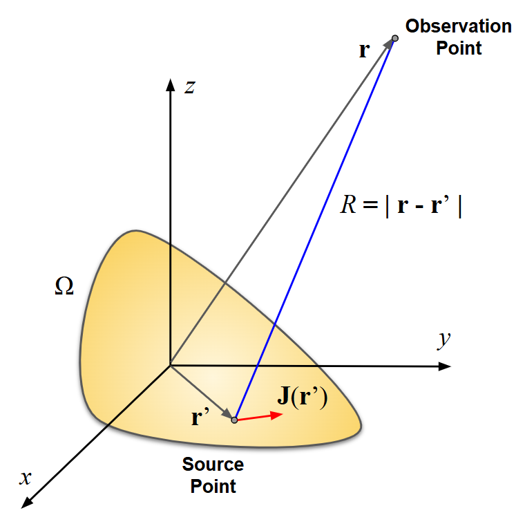
The general scenario is illustrated in Fig. 1: a current density distribution $\mathbf{J}(\mathbf{r}’)$ exists at source points $\mathbf{r}’$ within a volume $\Omega$, and we seek to determine the resulting $\mathbf{E}$ and $\mathbf{H}$ fields at observation points $\mathbf{r}$. To do this, we compute the distance between source and observation points,

$\displaystyle R \,=\, |\mathbf{r} \,-\, \mathbf{r}’|$,

and integrate over the source region $\Omega$ with differential volume elements $d^3r’$.

By substituting the Green’s function (11) into the potential expressions (12) and (13), applying the continuity equation (2) in (13), and finally using (4) and (6) to calculate the fields from the potentials, we obtain:

$\displaystyle \mathbf{E}(\mathbf{r}) \,=\, – \, \frac{j \omega \mu_0}{4 \pi} \iiint_\Omega \mathbf{J}(\mathbf{r}’) \, \frac{e^{-jkR}}{R} \, d^3r’ \,-\, \frac{j}{4 \pi \omega \varepsilon_0} \iiint_\Omega \nabla’ \cdot \mathbf{J}(\mathbf{r}’) \, \nabla \!\left(\frac{e^{-jkR}}{R}\right) d^3r’ \quad (14)$

$\displaystyle \mathbf{H}(\mathbf{r}) \,=\, \frac{1}{4 \pi} \iiint_\Omega \mathbf{J}(\mathbf{r}’) \times \nabla \!\left(\frac{e^{-jkR}}{R}\right) d^3r’ \qquad (15)$

Here, $\nabla’$ denotes derivatives with respect to the source coordinates $\mathbf{r}’$, while $\nabla$ denotes derivatives with respect to the observation coordinates $\mathbf{r}$.

Expression (14) will be used frequently to compute the electric field generated by current distributions in conductors, which is the typical scenario in transmitting antennas. The magnetic field may be obtained directly from (15), or alternatively via Faraday’s law (1.1.32) by applying the curl operator to the already calculated $\mathbf{E}$ field.

It is often desirable to avoid the derivatives of the current density $\mathbf{J}$ that appear in (14). By taking the gradient of the Lorenz gauge condition (8), the electric field can be written as

$\displaystyle \mathbf{E} \,=\, – \, j \omega \mathbf{A} \,-\, \frac{j}{\omega \mu_0 \varepsilon_0} \, \nabla (\nabla \cdot \mathbf{A}) \qquad (16)$

Thus, the calculation of the electromagnetic fields reduces to determining only the vector potential $\mathbf{A}$, from which the electric and magnetic fields follow using (16) and (4), respectively.

Substituting (12) into (16), we obtain

$\displaystyle \mathbf{E}(\mathbf{r}) = – \, \frac{j \omega \mu_0}{4 \pi} \iiint_\Omega \mathbf{J}(\mathbf{r}’) \, \frac{e^{-jkR}}{R} \, d^3r’ \,-\, \frac{j}{4 \pi \omega \varepsilon_0} \iiint_\Omega \left(\mathbf{J}(\mathbf{r}’) \cdot \nabla \right) \nabla \!\left(\frac{e^{-jkR}}{R}\right) d^3r’ \quad (17)$

To evaluate the fields in (15) and (17), we need the gradient of the Green’s function. Since it depends only on the distance between the observation point and the source point, we set up a spherical coordinate system with the origin at the source point. In this system, $R$ is the radial distance, and applying the gradient formula for a scalar field (1.2.2) yields

$\displaystyle \nabla \!\left( \frac{e^{-jkR}}{R} \right) \,=\, \frac{\mathbf{r} \,-\, \mathbf{r}’}{|\mathbf{r} \,-\, \mathbf{r}’|} \; \frac{\partial}{\partial R} \left( \frac{e^{-jkR}}{R} \right)$.

Hence,

$\displaystyle \nabla \!\left( \frac{e^{-jkR}}{R} \right) \,=\, – \, \frac{\mathbf{r} \,-\, \mathbf{r}’}{|\mathbf{r} \,-\, \mathbf{r}’|} \; \left( \frac{1}{R^2} + \frac{jk}{R} \right) e^{-jkR} \qquad (18)$

If the observation point is sufficiently far from the source region $\Omega$ such that $R$ is much greater than the maximum dimension of $\Omega$, the $1/R^2$ term in (18) can be neglected compared to the $1/R$ term. Under this far-field condition, the second integral in (17), which represents the conservative contribution of the field associated with $-\nabla V$, contains higher-order derivatives of the Green’s function and decays as $1/R^2$ or $1/R^3$. This term can therefore be neglected. Consequently, in the far-field region, the electric field is well approximated solely by the dissipative term proportional to the vector potential:

$\displaystyle \mathbf{E} \, \approx \, – \, j \omega \mathbf{A} \qquad \text{(far-field region)} \qquad (19)$

and the magnetic field in (4) can be approximated by (1.3.6), previously derived for point sources.

At this stage, we have all the analytical tools needed to compute the electromagnetic fields of antennas given their current density distribution. We now turn to the simplest possible case: the Hertzian dipole.

Fields of the Hertzian Dipole

With the expressions derived in (17) for the electric field and (15) for the magnetic field of an arbitrary current density distribution in free space, obtaining the fields of a Hertzian dipole becomes straightforward.

First, we define the Hertzian dipole. It is an elementary current element of amplitude $I$ (in Amperes) and infinitesimal length $dl$, with a specific orientation in space. Mathematically, we can model it as a current density $\mathbf{J}$ (A/m²) flowing along a cylindrical region with infinitesimal cross-sectional area $ds$ and infinitesimal length $\mathbf{dl} = \mathbf{\hat{dl}} \; dl$, where $\mathbf{\hat{dl}}$ is a unit vector that specifies the orientation of the element. If the current density $\mathbf{J} = \mathbf{\hat{dl}} \; J$ flows normally to the cross section, the total current is $I = J \, ds$. Since the differential volume element is $d^3r = ds \, dl$, we obtain:

$\displaystyle \mathbf{J}\, d^3r \,=\, \mathbf{\hat{dl}} \; J \, ds \, dl \,=\, \mathbf{\hat{dl}} \; I \, dl \qquad (20)$

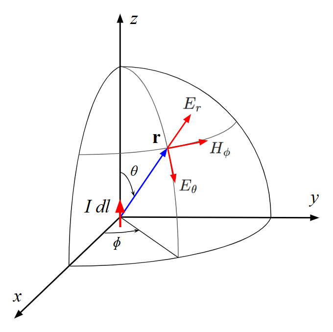
Let us assume that the current element is located at the origin, oriented along the $z$-axis, and that we have adopted a spherical coordinate system referenced to Cartesian axes as shown in Fig. 2. In this case, $\mathbf{\hat{dl}} = \mathbf{\hat{z}}$, and (20) reduces to:

$\displaystyle \mathbf{J}\, d^3r \,=\, \mathbf{\hat{z}} \; I \, dl \qquad (21)$

The oscillatory nature of this dipole follows from the continuity equation, which simplifies to $I = -dq/dt$. This corresponds to two charges $\pm q$ separated by the infinitesimal distance $dl$ along the $z$-axis, with alternating sign at angular frequency $\omega$ (since we are working with time-harmonic fields). In phasor form, the continuity equation becomes $I = -j \omega \, q$.

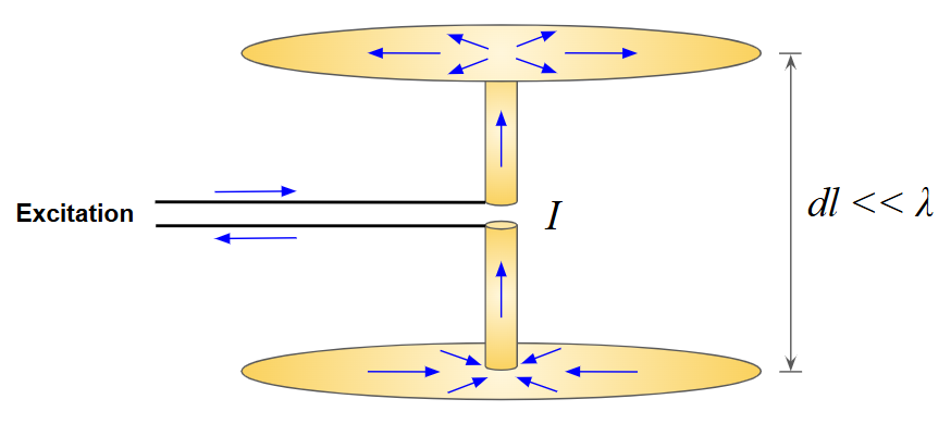
Although the Hertzian dipole is an idealized abstraction, it can be approximated in practice. One common implementation is a very short conducting rod (compared to the wavelength) connected to two circular plates placed at its ends, oriented perpendicular to the rod axis. The plates act like a capacitor, ensuring that the current along the rod remains nearly uniform. The entire structure must be made of a good conductor at the operating frequency so that ohmic losses can be neglected. Figure 3 illustrates this configuration. In this arrangement, the currents on the upper and lower plates flow in opposite directions, and their radiated fields largely cancel at distances beyond a fraction of a wavelength. Thus, for practical purposes, only the vertical current along the short rod contributes to radiation. Therefore, while $dl$ is treated as an infinitesimal length in the mathematical model, in practice it represents a finite but electrically small length compared to the wavelength.

The derivation of the fields radiated by the current element (21), in the coordinate system of Fig. 2, follows directly from (17) and (15). Since the current is constant and the source region $\Omega$ reduces to an infinitesimal volume, no actual integration is needed. Using also the gradient of the Green’s function from (18), the resulting electric and magnetic field components of the Hertzian dipole can be obtained. The final expressions are left as an exercise to the reader:

$\displaystyle E_r \,=\, \frac{k}{2 \pi} \, Z_{w0} \, I \, (k dl) \left( \frac{1}{(k r)^2} \,-\, \frac{j}{(kr)^3} \right) e^{- j k r} \, \cos{\theta} \qquad (22)$

$\displaystyle E_\theta \,=\, \frac{k}{4 \pi} \, Z_{w0} \, I \, (k dl) \left( \frac{j}{kr} \,+\, \frac{1}{(kr)^2} \,-\, \frac{j}{(kr)^3} \right) e^{- j k r} \, \sin{\theta} \qquad (23)$

$\displaystyle H_\phi \,=\, \frac{k}{4 \pi} \, I \, (k dl) \left( \frac{j}{kr} \,+\, \frac{1}{(kr)^2} \right) e^{- j k r} \, \sin{\theta} \qquad (24)$

where $Z_{w0} = \sqrt{\mu_0/\varepsilon_0} \approx 377 \; \Omega$ is the free space wave impedance. The remaining field components are all zero: $E_\phi = 0$, $H_r = 0$, and $H_\theta = 0$, owing to the convenient choice of a vertically oriented dipole. Thus, expressions (22)–(24) allow us to compute the electromagnetic field radiated by a Hertzian dipole at an observation point $(r, \theta, \phi)$, in accordance with the dipole orientation and coordinate system shown in Fig. 2, which also indicates the nonzero field components at the observation point.

We have deliberately written the dipole length $dl$ and the observation distance $r$ multiplied by the wavenumber, $k = 2\pi/\lambda$. In this form, both the dipole length and the observation distance can be normalized to the wavelength, since $kdl = 2\pi (dl/\lambda)$ and $kr = 2\pi (r/\lambda)$. This formulation clarifies our earlier assumption that $dl \ll \lambda$, or equivalently $dl/\lambda \ll 1$. The normalized distance $r/\lambda$ will later serve to define the different field regions surrounding the Hertzian dipole.

Finally, it should be noted that since the current amplitude $I$ is expressed as a phasor, if it represents an RMS value, then the field quantities given in (22)–(24) must also be interpreted as RMS values.

Near-Field and Far-Field Regions

The terms that depend on distance, appearing in parentheses in (22)–(24), are arranged in decreasing order of dominance as the observation distance from the Hertzian dipole increases: from the $1/r$ term, to the $1/r^2$ term, and finally the $1/r^3$ term. The $1/r$ term corresponds to the radiation field. We have already encountered this term in the study of point sources, where it emerges naturally as the spherical wave solution of the Helmholtz (vector wave) equation.

When the observation point is very close to the dipole, the dominant components of the electric field are $E_r$ and $E_\theta$, which vary as $1/r^3$. This field has the same structure as the static dipole field produced by two charges $+q$ and $-q$ aligned along the $z$-axis. For this reason, the near-field region is often referred to as the quasi-static region, since the field equations are identical to those of a static dipole, except that the charges now vary harmonically with time. The electric field also contains a transition term proportional to $1/r^2$, which smoothly connects the quasi-static near-field region with the far-field region.

A similar observation applies to the magnetic field: the $1/r^2$ term of $H_\phi$ corresponds to the well-known Biot–Savart law for a filamentary current of intensity $I$. The associated field lines form closed loops encircling the current axis.

These observations raise the question of whether “boundaries” can be rigorously defined between the different regions. From a mathematical standpoint, the fields are continuous functions of distance, and no sharp boundaries exist. Any definition of field regions is therefore conventional and depends on the level of approximation or accuracy that one is willing to accept when comparing terms.

A traditional approach is to define the boundary between the near- and far-field regions as the distance at which the $1/r$ and $1/r^2$ terms are equal:

$\displaystyle \frac{1}{kr} \,=\, \frac{1}{(kr)^2} \quad \implies \quad kr = 1$.

Since $k = 2\pi/\lambda$, this gives:

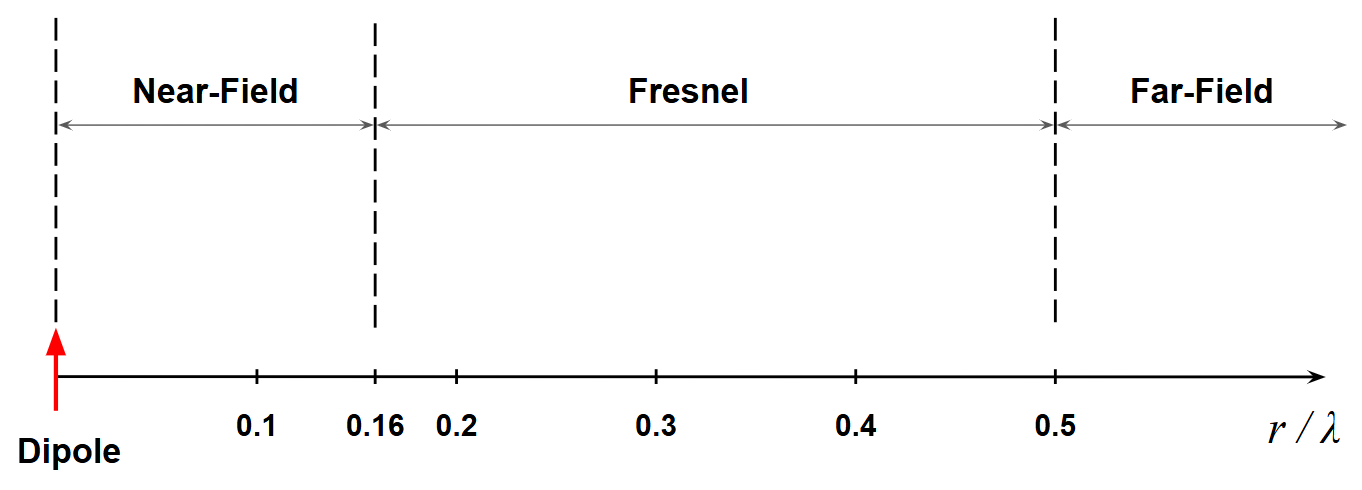
$\displaystyle r \,=\, \frac{\lambda}{2\pi} \approx 0.16\,\lambda \qquad (25)$

This expression is conventionally adopted as the boundary between near and far fields for a Hertzian dipole, and by extension, for any short antenna. Notably, this distance is independent of the antenna’s physical size.

However, because (25) merely marks the point where two terms are equal, a more conservative criterion is often applied: the far-field region is taken to begin at distances at least ten times larger, leaving an intermediate transition region known as the Fresnel zone. Yet, as we will see below, this criterion is too conservative, and a more practical choice is to place the boundary at half a wavelength, $r = \lambda/2$. Figure 4 illustrates a possible division into three field regions for the Hertzian dipole.

When studying the isotropic radiator in Section 1.2, we defined the wave impedance as the ratio of the electric to the magnetic field intensities for a TEM spherical wave. This results in a constant real value of $Z_{w0} \approx 377 , \Omega$, equal to the characteristic impedance of free space. If we retain only the $1/r$ terms of the fields, we can confirm this by dividing (23) by (24).

More generally, we can apply the same definition of wave impedance not only in the far field but also in the near-field region, across all distances. In this case, the wave impedance becomes a complex quantity that depends on distance. After rearranging the terms, we obtain:

$\displaystyle Z_w(kr) \,=\, \frac{E_\theta}{H_\phi} \,=\, Z_{w0} \left( \frac{(kr)^2}{1 + (kr)^2} \,-\, j \, \frac{1}{kr \, (1 + (kr)^2)} \right) \qquad (26)$

As we can see, the wave impedance satisfies:

$\displaystyle \lim_{kr \,\to\, \infty} Z_w(kr) \,=\, Z_{w0} \qquad (27)$

This property holds not only for the Hertzian dipole but for any antenna in free space. The wave impedance can thus be defined as the ratio of the electric and magnetic field components that are perpendicular to each other and transverse to the radial direction of propagation. A wave impedance close to $Z_{w0}$ indicates an almost TEM spherical wave with in-phase field components, which characterizes the far-field region.

It is instructive to plot the wave impedance of the Hertzian dipole as given by (26). Figure 5 shows the magnitude and phase of $Z_w$ as a function of the normalized distance $r/\lambda$. The “boundary” between the near- and far-field regions, defined by (25), is also marked for reference. This plot was generated using a GNU Octave script, available for download via the button below Fig. 5.

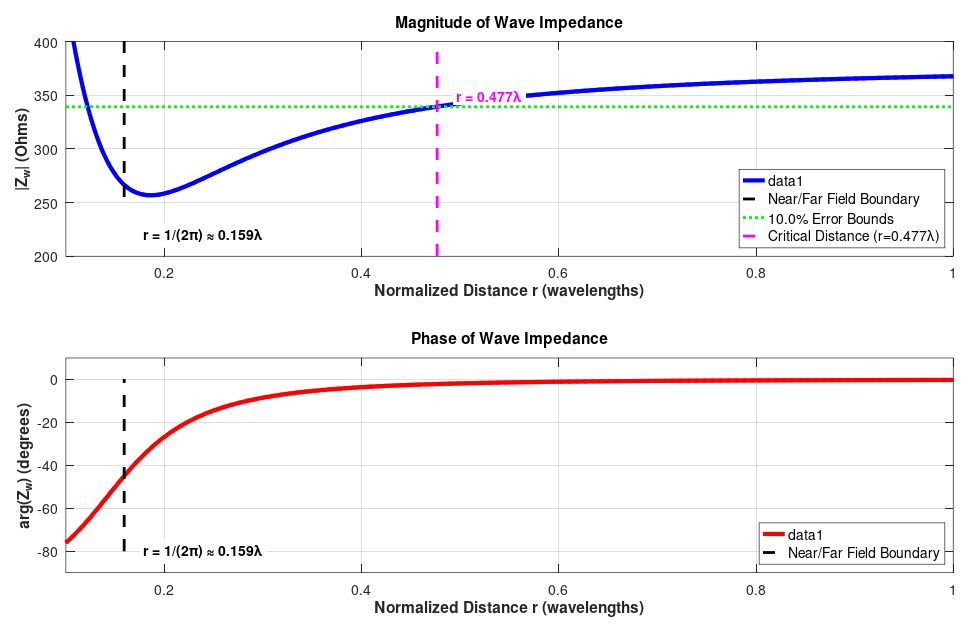
The script allows the user to specify a percentage error for $|Z_w|$ relative to $377\,\Omega$ and then calculates the distance $r/\lambda \geq 1/(2 \pi)$ at which the wave impedance falls within this tolerance. For example, with a 10% error, the script returns:

|Zw| reaches 377 ± 10.0% at r = 0.4766 wavelengths

Wave Impedance Characteristics:
Near-field boundary: r = 1/(2π) ≈ 0.1592 wavelengths
Far-field impedance: 377 Ohms (free space impedance)
Near-field impedance: capacitive (phase ≈ -90°)

At near-field boundary (r = 0.1592λ):
|Zw| = 266.3 Ohms
arg(Zw) = -44.8 degrees

At r = 0.5λ:
|Zw| = 342.5 Ohms
arg(Zw) = -1.8 degrees

At r = 1λ:
|Zw| = 367.7 Ohms
arg(Zw) = -0.2 degrees

Error Analysis (10.0% tolerance):
|Zw| first reaches 377 ± 37.7 Ohms at r = 0.4766λ (r ≥ 1/(2π))
At this distance:
  |Zw| = 339.4 Ohms
  arg(Zw) = -2.1 degrees
  Actual error: 37.59 Ohms (9.97%)

This suggests that, using a 10% tolerance criterion, a more practical boundary between the near- and far-field regions is located at approximately half a wavelength from the dipole.

By calculating the argument of the complex wave impedance, we obtain

$\displaystyle \arg(Z_w) \,=\, \arctan\!\left(\frac{\operatorname{Im}(Z_w)}{\operatorname{Re}(Z_w)}\right) \,=\, – \, \arctan\!\left(\frac{1}{(kr)^3} \right)$.

Thus, at large distances the wave impedance approaches a zero phase angle, while at short distances it tends toward $-\pi/2$, corresponding to a capacitive reactance, as illustrated in Fig. 5. This explains why the near-field region is often called the reactive near field. The Fresnel region, which serves as the transition zone, is also referred to as the radiative near field.

A more detailed discussion of wave impedance and the determination of near- and far-field boundaries is presented in the article: Wave Matching Coefficient: Defining the Practical Near-Far Field Boundary. There, a coefficient in decibels (dB), called the Wave Matching Coefficient (WMC), is introduced, derived from the wave impedance. This coefficient makes it possible to define a practical boundary between field regions based on a chosen tolerance in dB, analogous to return loss in transmission lines. Examples are given for both short and long antennas, demonstrating the generality of this method. The article also provides a calculator to apply the standard textbook formulas for near- and far-field boundary calculations.

It is worth mentioning another criterion for defining the onset of the far-field region of antennas: the curvature of the wavefront. In the Fresnel region, the wavefront is strongly curved (spherical), and the electric and magnetic fields are complex, lacking a stable, fixed relationship. At greater distances, the wavefront flattens. While it remains technically spherical, the curvature becomes negligible over the aperture of a receiving antenna, so it can be treated as a plane wave for practical purposes. This transition from a spherical to an effectively planar wavefront is directly linked to the concepts introduced by Joseph von Fraunhofer. The Fraunhofer criterion evaluates the maximum phase error of a spherical wave at the edge of an antenna compared to that of an ideal plane wave at the center. This consideration is particularly important for electrically large antennas. For this reason, the far-field region is also often called the Fraunhofer region.

Radiation Pattern and Field Representation

In the far-field region, the electric and magnetic fields of a Hertzian dipole are given by the $1/r$ terms of (23) and (24), respectively:

$\displaystyle E_\theta \,=\, \frac{j k}{4 \pi} \, Z_{w0} \, I \, (k dl) \frac{e^{- j k r}}{kr} \, \sin{\theta} \qquad (28)$

$\displaystyle H_\phi \,=\, \frac{E_\theta}{Z_{w0}} \qquad (29)$

From these expressions, the field pattern is obtained as

$\displaystyle f(\theta) \,=\, \sin{\theta} \qquad (30)$

We already employed this field pattern when analyzing arrays of point sources in Section 1.3. The radiated field is linearly polarized in the vertical plane, or the $\mathbf{\hat{\theta}}$ direction, which is the plane of the electric field. The resulting radiation pattern has a donut shape: it is maximum in the $xy$-plane (perpendicular to the dipole axis) and vanishes along the $z$-axis (the dipole axis itself). All field components in (22)–(24) exhibit rotational symmetry, meaning they do not depend on the azimuth angle $\phi$, as expected for a dipole oriented along the $z$-axis.

It is customary to represent field patterns in decibels. This requires first normalizing the field pattern in the range $0 \leq f(\theta) \leq 1$, and then applying the definition

$\displaystyle f_{dB}(\theta) \,=\, 20 \, \log \big| f(\theta) \big| \,\, (dB) \qquad (31)$

Here, the maximum value (equal to 1 after normalization) corresponds to 0 dB, while lower values appear as negative levels relative to this maximum. Since the logarithm tends to $-\infty$ at the nulls of the pattern, in practice the decibel scale is truncated at some lower bound, often -50 dB or -100 dB. For example, if the minimum is set to -100 dB, every value below this threshold is clipped at -100 dB.

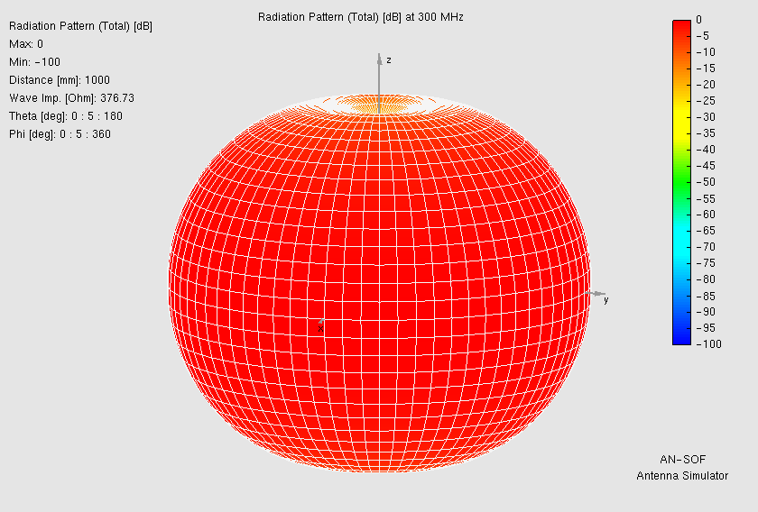
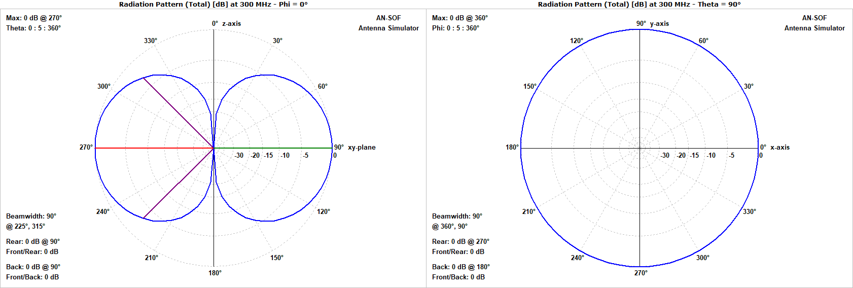
Figure 6 shows the 3D radiation pattern of a Hertzian dipole in decibels. It is also common to plot 2D cuts (slices) of the 3D pattern: a vertical slice and a horizontal slice. The vertical slice, which corresponds to the plane of the electric field (polarization), is known as the E-plane, while the horizontal slice is called the H-plane (Fig. 7).

Power Density and Radiated Power

From the far-field expressions of the electric and magnetic fields in (28) and (29), respectively, the power density points radially outward. Its radial component, expressed in terms of RMS field values, is

$\displaystyle S_r \,=\, \operatorname{Re}(E_\theta \, H^*_\phi) \,=\, Z_{w0} \, \left(\frac{|I| \, kdl}{4 \pi}\right)^2 \, \frac{\sin^2{\theta}}{r^2} \qquad (32)$

This expression highlights two key features: the inverse-square law dependence on distance, and the radiation pattern, given by

$\displaystyle F(\theta) \,=\, f^2(\theta) \,=\, \sin^2{\theta} \qquad (33)$

which is simply the square of the field pattern defined in (30). The radiation pattern in decibels is then defined as

$\displaystyle F_{dB}(\theta) \,=\, 10 \, \log{\big| F(\theta) \big|} \,\, (dB) \qquad (34)$

By substituting (33) into (34), we obtain the same result as in (31). Thus, the field pattern and the radiation pattern coincide when expressed in decibels. For this reason, in Fig. 6 we referred to the decibel-scaled field pattern as the “radiation pattern.”

To calculate the total power radiated by the Hertzian dipole, we follow the same procedure used for the isotropic radiator. Using the general expression for radiated power in (1.2.15), we integrate the radial power density over the surface of a sphere centered at the dipole:

$\displaystyle P_r \,=\, \int_0^{2 \pi} d\phi \int_0^\pi S_r \, r^2 \, \sin{\theta}\, d\theta \qquad (35)$

Substituting (32) into (35) and carrying out the integrations yields

$\displaystyle P_r \,=\, 20\,|I|^2 (k dl)^2 \qquad (36)$

where we have used the approximation $Z_{w0} \approx 120 \pi \, \Omega$ for the free-space wave impedance. The radiated power depends on the square of the current amplitude, $|I|^2$. This dependence leads directly to the important concept of radiation resistance in antenna theory.

Radiation Resistance of the Hertzian Dipole

Returning to the physical realization of the Hertzian dipole shown in Fig. 3, let us assume there are no power losses in the system. All conductors, including the transmission line feeding the dipole, are perfect, and the line is perfectly matched. Under these conditions, all the input power delivered by the source at the transmission line input reaches the dipole feedpoint, where it is entirely radiated into space.

From the perspective of the feedpoint terminals, the current $I$ flowing into the dipole encounters a resistance, since real power is “consumed.” However, this power is not dissipated as heat (ohmic losses), but rather radiated outward. This leads to the definition of the radiation resistance, the effective resistance that accounts for radiated power:

$\displaystyle R_r \,=\, \frac{P_r}{|I|^2} \qquad (37)$

This represents the resistance at which the same amount of power would be dissipated if it were a conventional resistor. Substituting the radiated power expression from (36) into (37), we obtain

$\displaystyle R_r \,=\, 20 \,(kdl)^2 \,=\, 80 \pi^2 \left(\frac{dl}{\lambda}\right)^2 \qquad (38)$

It is evident that the radiation resistance of a Hertzian dipole is very small, since $dl \ll \lambda$ is the underlying assumption of this model. Nevertheless, as the dipole length increases, its radiation resistance grows rapidly, proportional to the square of the length. Of course, expression (38) is no longer valid once the dipole length approaches roughly one-tenth of a wavelength.

Understanding radiation resistance is essential because it directly influences impedance matching at the feedpoint and plays a central role in determining antenna efficiency, a concept we will define shortly.

Directivity and Beamwidth

Up to this point, we have introduced key parameters and quantities as needed to describe antenna behavior. Now it is time to define directivity, one of the most fundamental measures of antenna performance.

As we have seen, an isotropic radiator (one that radiates equally in all directions) cannot physically exist. Real antennas inherently exhibit nulls in certain directions while concentrating energy in others. To quantify this concentration of radiated power, we define the directivity of an antenna as the ratio of the maximum power density to the average power density over all directions:

$\displaystyle D \,=\, \frac{S_{\max}}{S_{\text{av}}} \quad (39)$

Here, $S_{\text{av}}$ is the average (in space) power density. Since the fields are assumed to be time-harmonic, the power density is already time-averaged. To obtain the spatial average, we integrate the radial component of the Poynting vector over the surface of a sphere $S_p$ that encloses the antenna and then divide by the surface area of the sphere. For a sphere of radius $r$:

$\displaystyle S_{\text{av}} \,=\, \frac{1}{4\pi r^2} \iint_{S_p} \mathbf{S} \cdot d^2\mathbf{r} \quad (40)$

The surface integral is simply the total radiated power $P_r$, so:

$\displaystyle S_{\text{av}} \,=\, \frac{P_r}{4\pi r^2} \quad (41)$

This expression is quite general and not limited to the Hertzian dipole. Substituting (41) into (39), and specifying that the maximum power density must be taken in the far-field region, we arrive at the general definition of directivity:

$\displaystyle D \,=\, \frac{4\pi}{P_r} \, \lim_{r \, \to \, \infty} r^2 S_{\max} \quad (42)$

For the Hertzian dipole, the maximum power density occurs at $\theta = \pi/2$, as given in (32). Using the radiated power derived in (36), we obtain:

$\displaystyle D \,=\, \frac{Z_{w0}}{80\pi} \,=\, 1.5 \quad (43)$

where we have used the approximation $Z_{w0} \approx 120\pi \, \Omega$. Thus, the directivity of a Hertzian dipole is a constant value of 1.5, independent of the dipole’s physical size.

It is instructive to calculate the directivity of an isotropic radiator. Since it radiates the same power density in all directions, its maximum power density is equal to its average value, and therefore the directivity of an isotropic source is 1. This provides an alternative way to interpret directivity: a Hertzian dipole with a directivity of 1.5 means it concentrates 50% more power in its strongest direction compared to an isotropic radiator that radiates the same total power.

In this sense, directivity can be understood as a measure of directionality relative to isotropy. For this reason, the definition of directivity we introduced is often referred to as directivity with respect to an isotropic source.

When directivity is expressed in decibels, the unit is written as dBi (decibels relative to an isotropic radiator):

$\displaystyle D_{\mathrm{dBi}} \,=\, 10 \, \log(D) \,\, \text{(dBi)} \qquad (44)$

Then, the directivity of a Hertzian dipole in decibels relative to an isotropic radiator is

$\displaystyle D_{\mathrm{dBi}} \,=\, 10 \, \log(1.5) \,=\, 1.76 \, \text{dBi}$.

Expressing directivity in dBi makes it easier to compare antennas. For example, if antenna $A$ has a directivity of $D_A \, \text{(dBi)}$ and antenna $B$ has a directivity of $D_B \, \text{(dBi)}$, then the directivity of A with respect to B in decibels is simply: $D_A \,-\, D_B$.

Another important metric related to directionality is the beamwidth. It is defined as the angular width of the main lobe of a radiation pattern. Typically, the beamwidth is measured on a 2D slice of the radiation pattern, as shown in Fig. 7.

In the left panel of Fig. 7, we see the E-plane polar diagram of a Hertzian dipole. The figure includes lines indicating the beamwidth, and the legend at the lower left corner states: “Beamwidth: 90°.”

This beamwidth is obtained by locating the two directions on either side of the main lobe maximum where the radiation intensity falls to half its peak value. Equivalently, in decibel scale, the radiation pattern decreases by 3 dB at these points. These directions are known as the half-power directions, and the corresponding angular separation is called the half-power beamwidth (HPBW) of the antenna.

To calculate the HPBW of the Hertzian dipole, we start with its radiation pattern given by (33). Setting the pattern equal to $1/2$ gives an equation in $\theta$:

$\displaystyle \sin^2 \theta \,=\, \frac{1}{2} \quad \implies \quad \theta \,=\, \frac{\pi}{4} \,=\, 45^\circ$

Since the main lobe extends symmetrically on both sides of the maximum, the HPBW is twice this value:

$\displaystyle \text{HPBW} \,=\, 90^\circ \qquad (45)$

Equivalent Circuit Model of a Hertzian Dipole

From the perspective of its feedpoint, a Hertzian dipole presents both a radiation resistance and a reactance. The reactance accounts for the reactive energy stored in the dipole’s near field. If we physically realize a Hertzian dipole by attaching parallel plates at its ends (as illustrated in Fig. 3), the reactance will be negative (capacitive in nature) and much larger in magnitude than the radiation resistance. We denote this reactance as

$\displaystyle X_a \,=\, – \, \frac{1}{\omega \, C_a} \qquad (46)$

where $C_a$ is the effective capacitance, which can be approximated using the parallel-plate capacitor formula:

$\displaystyle C_a \,=\, \varepsilon_0 \, \frac{A}{dl}$,

with $A$ the plate area and $dl$ the dipole length (i.e., the separation between plates). This approximation holds provided the plate dimensions are much larger than $dl$. Thus, the Hertzian dipole can be viewed as a small free-space capacitor, and the radiation we compute is the minute amount normally neglected in circuit theory. However, this radiation becomes non-negligible once the physical size of the system approaches about 1% of a wavelength or larger.

Now let us account for losses. Since we are mainly interested in the dipole itself, we neglect ohmic losses in the plates but not in the conducting arms of the dipole. If the dipole is modeled as a cylindrical conductor of radius $a$ and conductivity $\sigma$ (S/m) (Siemens per meter), the resistance per unit length due to skin effect is:

$\displaystyle R_i \,=\, \frac{1}{2 \pi a} \, \sqrt{\frac{\mu_0 \omega}{2 \sigma}} \quad \left(\frac{\Omega}{\text{m}}\right) \qquad (47)$

For copper, the conductivity is approximately $\sigma \approx 5.8 \times 10^7 \, \text{S/m}$. The reciprocal of conductivity, $1/\sigma$, is the resistivity, a quantity often tabulated for common materials.

Since the Hertzian dipole carries a uniform current distribution along its length $dl$, the effective resistance appearing at the feedpoint due to ohmic losses is simply:

$\displaystyle R_L \,=\, R_i \, dl \qquad (48)$

This is known as the loss resistance.

We now have all components needed to construct an equivalent circuit for the Hertzian dipole, shown schematically in Fig. 8. Its feedpoint impedance is:

$\displaystyle Z_a \,=\, R_r \,+\, R_L \,+\, j X_a \qquad (49)$

where

• $R_r$ is the radiation resistance given by Eq. (38),
• $R_L$ is the loss resistance given by Eq. (48), and
• $X_a$ is the reactive component given by Eq. (46).

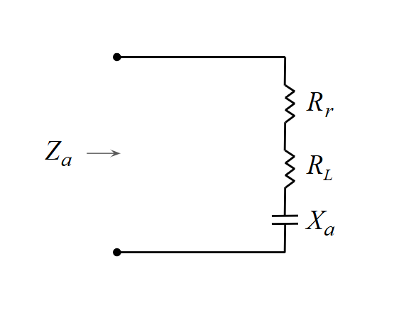
In practice, to operate a physical Hertzian dipole, a tuning inductor is needed to cancel the capacitive reactance $X_a$, along with an impedance matching network to match $\operatorname{Re}(Z_a) = R_r + R_L$ to a standard transmission line impedance (commonly 50 or 75 Ω).

If the RMS input current is $I$, then:

• The input power is

$\displaystyle P_{\text{in}} \,=\, |I|^2 \, (R_r + R_L) \qquad (50)$

• The radiated power is

$\displaystyle P_r \,=\, |I|^2 \, R_r \qquad (51)$

• The lost power, dissipated as heat, is

$\displaystyle P_L \,=\, |I|^2 \, R_L \qquad (52)$

This sets the stage for the introduction of the concept of radiation efficiency.

Radiation Efficiency and Antenna Gain

In general, the efficiency of a system is defined as the ratio of useful power output to the total power supplied. For antennas, the useful output is the radiated power, since the purpose of an antenna is to transmit electromagnetic energy into space. Accordingly, we define the radiation efficiency as the ratio of the radiated power to the input power delivered to the antenna terminals:

$\displaystyle \eta \,=\, \frac{P_r}{P_{\text{in}}} \qquad (53)$

Using the input and radiated powers from the equivalent circuit of the Hertzian dipole in (50) and (51), the efficiency can be expressed in terms of circuit components as:

$\displaystyle \eta \,=\, \frac{R_r}{R_r \,+\, R_L} \qquad (54)$

As expected from energy conservation, the radiated power cannot exceed the input power, so the efficiency satisfies $0 \leq \eta \leq 1$. It is often expressed as a percentage by multiplying (53) by 100.

Previously, we defined directivity as the ratio of the maximum radiated power density in the far field to the average power density over a sphere of radius $r$. The average power density was obtained by dividing the total radiated power by the spherical surface area $4\pi r^2$.

In practice, however, the input power is usually the most accessible quantity, since it can be measured at the antenna terminals through voltage and current. If we use the input power instead of the radiated power to compute the average power density that would be achieved if all the input power were radiated, $P_{\text{in}}/(4 \pi r^2)$, we arrive at the definition of antenna gain:

$\displaystyle G \,=\, 4 \pi r^2 \, \frac{S_{\max}}{P_{\text{in}}} \qquad (55)$

or, more formally, as a far-field metric:

$\displaystyle G \,=\, \frac{4\pi}{P_{\text{in}}} \, \lim_{r \, \to \, \infty} \, r^2 \, S_{\max} \qquad (56)$

By comparing this with the directivity definition in (42), and applying the efficiency definition in (53), we obtain:

$\displaystyle G \,=\, \eta \, D \qquad (57)$

In decibel scale relative to isotropic (dBi), this becomes:

$\displaystyle G_{\text{dBi}} \,=\, D_{\text{dBi}} \,+\, 10 \, \log{\eta} \quad (\text{dBi}) \qquad (58)$

Since $0 \leq \eta \leq 1$, the second term in (58) is negative. Therefore, the gain is generally less than the directivity: $G \leq D$. Only in ideal, lossless antennas (or when losses are negligible) does the gain equal the directivity.

It is worth noting that the definitions we have adopted for directivity and gain are based only on the direction of maximum radiation, through the maximum power density $S_{max}$. For this reason, they are often referred to as peak directivity and peak gain. If, instead, we evaluate the power density in a direction other than the maximum, the resulting directivity and gain will depend on the observation angles $(\theta, \phi)$ in spherical coordinates. Furthermore, directivity and gain can also be expressed in terms of polarization components, by decomposing the radiation pattern into two orthogonal linear polarizations or into right- and left-hand circular polarizations, as we will see later.

Relating Electric Field Strength to Antenna Power and Gain

We are now in a position to derive some practical formulas that are frequently used in antenna engineering. In practice, it is often desirable to calculate the electric field strength produced by an antenna for a given input power, since the input power is a parameter that can be directly controlled and measured at the feedpoint.

For known antennas, the gain is typically specified, so having a formula that relates field strength in the far-field region to the input power and antenna gain is very useful.

For the Hertzian dipole, the RMS electric field strength is given by the magnitude of (28):

$\displaystyle |E_\theta| \,=\, 30 \, |I| \, k dl \, \frac{\sin{\theta}}{r} \qquad (59)$

where we have used the approximation $Z_{w0} \approx 120 \pi \, \Omega$.

Since the radiated power is $P_r = |I|^2 \, R_r$, and using the expression for the radiation resistance (38) together with the dipole’s directivity $D = 1.5$, it follows that:

$\displaystyle |E_\theta| \,=\, \frac{\sqrt{30 \, P_r \, D}}{r} \, \sin{\theta} \qquad (60)$

This gives the RMS electric field strength in terms of the radiated power. Introducing the gain as $G = \eta \, D$, with $\eta = P_r/P_\text{in}$, we finally obtain:

$\displaystyle |E_\theta| \,=\, \frac{\sqrt{30 \, P_\text{in} \, G}}{r} \, \sin{\theta} \qquad (61)$

Equation (61) expresses the far-field strength at a distance $r$ and observation angle $\theta$, as a function of the input power and antenna gain.

Historically, this formula was widely used for short antennas operating in the LF bands and became a standard tool for RF engineers in the early days of broadcasting during the mid-20th century. In the next section, we will present an online calculator based on this result for short dipoles.

What, Then, Is an Antenna?

Up to this point, we have followed a path that began with Maxwell’s equations, passed through the concepts of plane and spherical waves, and progressed to idealized radiators such as the isotropic point source and the Hertzian dipole. Along the way, we developed the tools to describe electromagnetic fields through potentials, we identified how power is distributed in space through radiation patterns, and we introduced key performance metrics such as directivity, gain, radiation resistance, and equivalent circuit representations.

At this stage, it is natural to ask: what is an antenna?

An antenna is a device designed to radiate or receive electromagnetic energy.

An antenna transforms electromagnetic energy confined and guided within a bounded region into propagating electromagnetic waves, and vice versa.

The Hertzian dipole has been our simplest model of an antenna. Despite being an idealized element of infinitesimal length, it already illustrates the fundamental mechanisms of radiation:

• Localized current acts as the source of electromagnetic waves.
• The resulting near field contains both reactive and radiative components.
• Beyond a certain distance, the field assumes the familiar spherical wave structure, characterized by a well-defined radiation pattern and wave impedance.
• Key antenna properties, such as directivity, gain, and radiation resistance, emerge naturally from this analysis.

From this perspective, every practical antenna, no matter how complex in geometry or design, can be viewed as a more elaborate realization of these same principles. The Hertzian dipole is not only a theoretical building block but also a conceptual anchor: it shows that the essence of an antenna lies in its role as a mediator between sources and fields, between circuits and space.

In the chapters that follow, we will move beyond this idealized model to analyze practical antenna types. Yet the insights gained from the Hertzian dipole will remain central: every antenna can be understood, at least in part, as a collection or extension of dipoles, governed by the same electromagnetic principles we have just explored.

Simulating a Hertzian Dipole in AN-SOF

Now that we have developed the theoretical foundations, it is time for a hands-on exercise with the AN-SOF Antenna Simulator. The reader can consult the documentation through these links:

• AN-SOF User Guide

• Quick Start Guide

We recommend reviewing the Simulation Setup chapter in the user guide and running at least the first example simulation from the quick start guide.

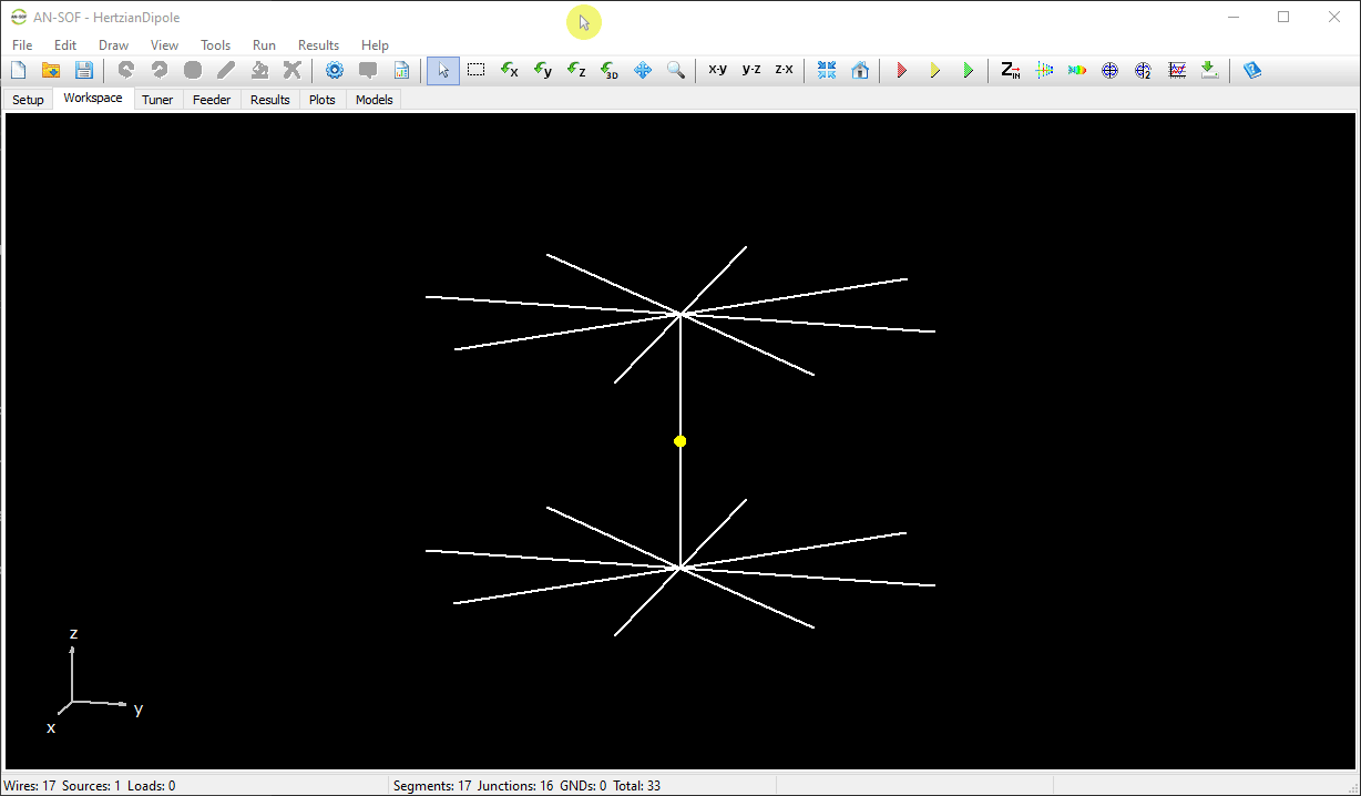
In AN-SOF we can build wire structures, which makes it possible to approximate a Hertzian dipole. Figure 9 shows such a model. The frequency is set to $300 \, \text{MHz}$, giving a wavelength of approximately 1 meter. The dipole length is chosen as 1% of the wavelength, i.e. $dl = 0.01\lambda$. The dipole itself is represented by a short vertical wire (aligned with the $z$-axis), while short horizontal radial wires are added at both ends to promote a nearly uniform current distribution, similar to the role of the plates in Fig. 3.

The precomputed model can be downloaded via the button below Fig. 9. Copper has been assigned as the material for all wires, so ohmic losses are included. The gain pattern shown in Fig. 9 is donut-shaped, as predicted theoretically, with a peak gain of 1.28 dBi. This is slightly below the theoretical 1.76 dBi of a lossless dipole. The difference of $1.76 \,-\, 1.28 = 0.48 \, \text{dB}$ can be attributed to ohmic losses. This is confirmed in the Results tab, where the radiation efficiency is $\eta \approx 90\%$, meaning about 10% of the input power is dissipated as heat.

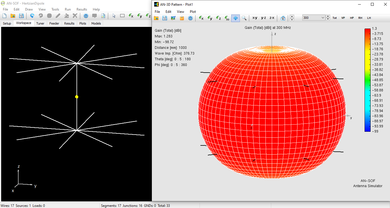
The Results tab also shows a directivity of 1.75 dBi, in excellent agreement with theory. Minor discrepancies arise from practical modeling considerations: AN-SOF represents wires with finite radii (the ideal Hertzian dipole assumes zero radius), and the radial wires should ideally be longer to further uniformize the current, though here we chose equal lengths for clarity.

The input impedance is reported as $Z_a \approx 0.08 \,-\, j \,1070 \; \Omega$, showing a very small resistance and a large capacitive reactance, consistent with theoretical expectations. The input resistance includes both radiation resistance and ohmic loss resistance, which cannot be separated directly. This separation is a theoretical construct, since it assumes that introducing losses does not alter the current distribution relative to the ideal lossless dipole.

However, because AN-SOF provides the radiated power, we can estimate the radiation resistance directly. Setting the input power to $100 \, \text{W}$ (for numerical convenience), the Power Budget in the Results menu reports $P_r \approx 89.9 \, \text{W}$. The input current can then be extracted by right-clicking the vertical wire, selecting List Currents, and pressing Current on Segment in the bottom toolbar, yielding $|I| = 35.2 \, \text{A}$. The radiation resistance is then

$\displaystyle R_r \,=\, \frac{P_r}{|I|^2} \,=\, \frac{89.9 \, \text{W}}{(35.2 \, \text{A} )^2} \,\approx\, 0.073 \, \Omega$,

which closely matches the analytical value from Eq. (38), $R_r = 0.079 \, \Omega$. Figure 10 provides an animation of the steps for accessing the Power Budget and retrieving the input current.

Conclusion

Through this simulation in AN-SOF we have confirmed the theoretical concepts studied for the Hertzian dipole. We observed that:

• The radiation pattern has the expected donut shape, with peak directivity close to the theoretical value.
• The simulated gain is lower than the theoretical directivity due to ohmic losses, yielding an efficiency of about 90%.
• The input impedance shows a small resistance and a large capacitive reactance, in agreement with theory.
• By combining radiated power and feed current from the simulator, we obtained a radiation resistance very close to the analytical result.

This exercise demonstrates how theoretical models translate into practical simulations, clarifies the impact of losses and geometry on antenna performance, and builds a bridge between mathematical derivations and engineering practice.

References

- J. A. Stratton, Electromagnetic Theory. New York, NY, USA: McGraw-Hill, 1941. ↩︎
- R. W. P. King, The Theory of Linear Antennas. Cambridge, MA, USA: Harvard University Press, 1956. ↩︎
- R. F. Harrington, Time-Harmonic Electromagnetic Fields. New York, NY, USA: IEEE Press/Wiley-Interscience, 2001 (Original work published 1961). ↩︎
- W. L. Stutzman and G. A. Thiele, Antenna Theory and Design, 3rd ed. Hoboken, NJ, USA: Wiley, 2012. ↩︎
- J. D. Kraus, Antennas, 2nd ed. New York, NY, USA: McGraw-Hill, 1988. ↩︎
- C. A. Balanis, Antenna Theory: Analysis and Design, 4th ed. Hoboken, NJ, USA: Wiley, 2016. ↩︎
- C. Capps, “Near field or far field?,” EDN, vol. 46, no. 18, pp. 95–102, Aug. 16, 2001. ↩︎