Search for answers or browse our Knowledge Base.
Guides | Models | Validation | Book
Advanced Modeling of Monopoles over Radial Wire Ground Screens
Explore the enhanced methodology for modeling LF/MF monopoles over radial wire ground screens. Learn how AN-SOF integrates Poynting’s theorem with the Exact Kernel to provide precise resistance and reactance calculations, validated against Professor James R. Wait’s classical analytical results. Essential for broadcast engineers seeking high-precision radiation efficiency and impedance matching data.
Monopole antennas have been a cornerstone of radio communications since the early 20th century, particularly within the LF (Low Frequency) and MF (Medium Frequency) bands. In broadcast applications, the ground is not merely a structural support but a functional component of the antenna system. Consequently, accurately predicting power losses in the Earth’s soil is vital, as these losses directly impact the antenna’s radiation efficiency and input impedance.
The Role of Radial Ground Screens
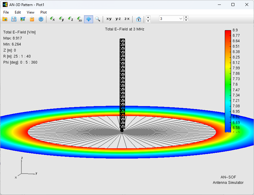
The input impedance of a monopole is sensitive to the electrical parameters of the soil in its immediate vicinity. Because natural soil often has poor conductivity, engineers install buried or surface-mounted radial wire screens to artificially enhance the ground’s performance (Fig. 1). These radials typically extend a quarter-wave ($\lambda/4$) or half-wave ($\lambda/2$) from the base of the monopole.
Because monopoles are linear structures, modeling them over a real ground plane involves applying theories originally developed for cylindrical antennas in free space. However, obtaining high-precision experimental data for these systems is challenging; LF/MF towers can reach heights of hundreds of meters, making controlled measurements difficult. Therefore, numerical simulation validated against established analytical models is the primary tool for design.
Comparative Methodologies: Wait vs. Dorado
Historically, two primary analytical approaches have dominated this field:
- Wait’s Method (1954): Professor James R. Wait developed a methodology based on surface impedance and a reaction integral formulation. His approach was comprehensive, allowing for the calculation of both the resistive (real) and reactive (imaginary) components of the antenna’s input impedance. Refer to “Impedance of a Top-Loaded Antenna of Arbitrary Length over a Circular Grounded Screen” by J.R. Wait and W.J. Surtees, Journal of Applied Physics (volume 25, page 553, 1954).
- Dorado’s Method (2006): This approach utilizes Poynting’s theorem to calculate the power lost in the soil analytically. While effective for determining the ground plane loss resistance, Dorado’s original methodology utilized the thin-wire approximation and was limited to calculating the resistance ($R$), leaving the reactance ($X$) undefined.
The AN-SOF Enhancement
AN-SOF improves upon these classical methods by integrating Poynting’s theorem with the Exact Kernel formulation. Unlike Dorado’s method, which relies on a thin-wire approximation that can lead to inaccuracies near the feed point, AN-SOF accurately incorporates the effect of the antenna’s finite radius.
Furthermore, AN-SOF provides a significant advantage over many simplified models by determining the full complex input impedance ($R + jX$). This allows us to design matching networks more accurately, ensuring maximum power transfer from the transmitter.
Validation and Results
The efficacy of the AN-SOF implementation is demonstrated by comparing its results with the analytical findings of Professor Wait.
Figure 2 illustrates the variation in input resistance ($\Delta R$), relative to a PEC ground plane, for a quarter-wave ($\lambda/4$) monopole antenna positioned above a radial wire ground screen. The study analyzes the increase in input resistance as a function of the screen radius for two different radial counts ($N = 20$ and $N = 100$), comparing results from AN-SOF, Wait, and Dorado.
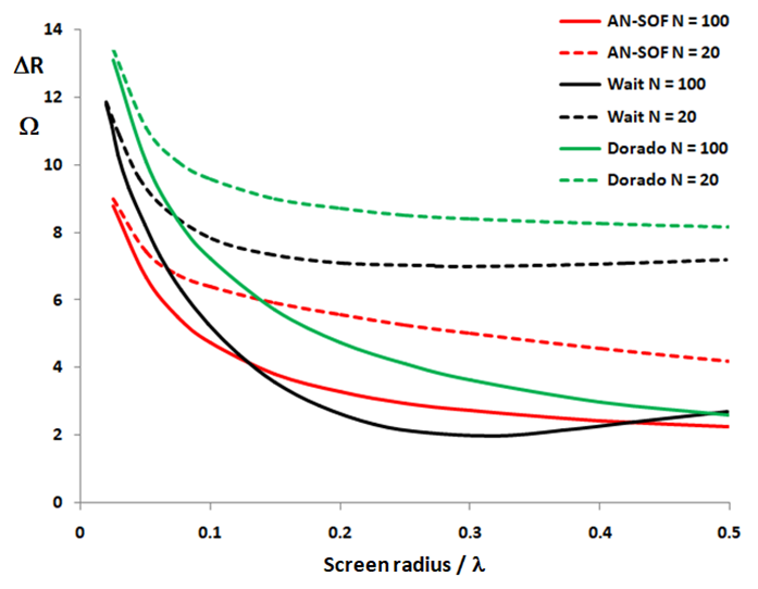
As illustrated in Fig. 2, the AN-SOF results exhibit a high degree of correlation with the findings of Wait and Dorado across various screen radii. This agreement is particularly noteworthy considering the computational constraints of the mid-20th century when Wait’s theory was developed. The convergence between numerical simulation and analytical theory confirms that AN-SOF provides a reliable, high-precision environment for modeling complex ground-screen interactions.
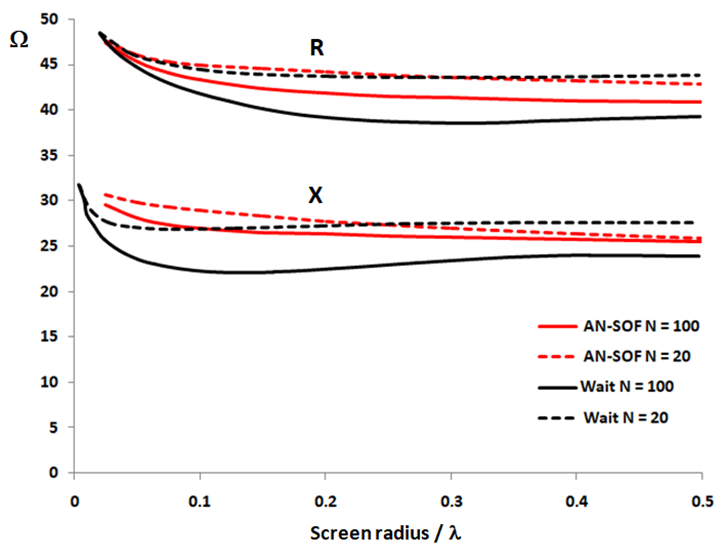
Figure 3 illustrates the input resistance ($R$) and reactance ($X$) of a quarter-wave monopole antenna over a radial wire ground screen. The results are plotted as a function of the screen radius (in wavelengths) for radial counts of $N = 20$ and $N = 100$. Once again, the agreement between the AN-SOF simulation and Wait’s analytical theory is remarkable.
Modeling Considerations
When using these models for LF/MF broadcast design, users should consider the following:
- Soil Parameters: Input accurate conductivity ($\sigma$) and permittivity ($\varepsilon_r$) for the specific site.
- Radial Density: As seen in the comparison between $N = 20$ and $N = 100$, increasing the number of radials stabilizes the input impedance and reduces ground loss.
- Exact Kernel Benefits: For thick radiating towers, the Exact Kernel ensures that the feedpoint impedance does not diverge as the mesh is refined, a common issue in legacy NEC-based solvers.
By leveraging these advanced methodologies, designers can optimize the number and length of radial wires to achieve the desired radiation efficiency while minimizing material costs.
Conclusions
The accurate characterization of monopole antennas above radial wire ground screens remains a fundamental challenge in broadcast engineering, particularly within the LF and MF bands. As demonstrated, the antenna’s efficiency and input impedance are inextricably linked to the electrical properties of the surrounding soil and the geometry of the grounding system.
By integrating the classical Poynting’s theorem with a modern Exact Kernel formulation, AN-SOF provides a robust bridge between theoretical analytical models and practical numerical simulation. This methodology effectively overcomes the limitations of legacy “thin-wire” approximations, which often struggle with convergence and feed-point singularities.
The high correlation between AN-SOF’s numerical results and Professor Wait’s established analytical data validates this enhanced approach. For the broadcast engineer, this precision offers a dual benefit: the ability to calculate full complex input impedance (both resistance and reactance) for superior matching network design, and the insight required to optimize ground screen configurations. Ultimately, these advanced modeling techniques allow for the design of more efficient, reliable, and cost-effective broadcast installations.
See Also:
Technical Keywords: Monopole Antenna, Radial Wire Ground Screen, LF/MF Broadcast, Ground Losses, James R. Wait Theory, Poynting’s Theorem, Exact Kernel, Radiation Efficiency, Input Impedance, Surface Impedance, Numerical Validation, Sommerfeld-Wait Model.
