Search for answers or browse our Knowledge Base.
Guides | Models | Validation | Book
Wave Matching Coefficient: Defining the Practical Near-Far Field Boundary
Discover how the Wave Matching Coefficient (WMC) redefines near-far field boundaries. Using a 20 dB threshold, we uncover new distances for elementary antennas and a consistent method to define non-spherical boundaries for antennas of any size or complexity relative to the wavelength.

In this article, we explore absolute wave impedance and the wave matching coefficient (WMC) as practical tools for defining the near-far field boundary of antennas of any size or complexity relative to the wavelength. By utilizing these measures, we gain a better understanding of wave propagation as a function of distance from the source antenna, employing a decibel scale that enables clearer visualization of significant changes in wave impedance. As a general guideline, a WMC value of 20 dB proves to be an appropriate threshold for distinguishing between the near and far field zones. Through examples involving both elementary and large-scale antennas relative to the wavelength, we observe that the 20 dB boundary is consistently located at a distance of λ/3 for elementary antennas, while it takes on an irregular and non-spherical shape for antennas of comparable size or greater than the wavelength.
Introduction
The determination of the far-field region of an antenna has been a topic extensively discussed in books and texts on antennas for nearly a century. However, it continues to spark debates even today. Identifying the regions surrounding an antenna is crucial for various applications, such as near-field measurements in an anechoic chamber to predict the far-field radiation pattern or in electromagnetic compatibility (EMC) to optimize shielding in the near-field region, minimizing interference.
Based on the observation of elementary electric or magnetic dipole fields, three distinct regions can be identified in terms of the distance, $r$, from the dipole:
- The reactive near-field region, where terms proportional to $1/r^3$ predominate.
- A transition region or Fresnel zone, where terms proportional to $1/r^2$ predominate.
- The far-field region or Fraunhofer zone, where terms proportional to $1/r$ predominate.
There is also a two-region model where the reactive near-field and the Fresnel zone are considered as part of the same near-field region. When antennas are more complex than elementary dipoles, it becomes nontrivial to identify the electromagnetic field zones. It is important to note that the definition of a boundary between the near-field and far-field regions is always arbitrary and depends on the acceptable margin of error in practice. There is no sharp edge or discontinuity between these regions; instead, the electromagnetic field initially behaves as a quasi-static field near the radiation source and gradually transforms into a Transverse Electromagnetic (TEM) wave with a spherical wavefront as the distance increases.
The Traditional Boundary Between Near Field and Far Field
In most textbooks, we can find that the far-field region begins at a distance from the antenna given by $2D^2/\lambda$, where $D$ is the maximum dimension of the antenna and $\lambda$ is the wavelength. This boundary between regions works reasonably well for cases of electrically large antennas, where $D \gg \lambda$. However, there are many exceptions to this rule, such as in the case of parabolic antennas where this boundary must be extended twofold. For electrically small antennas, where $D \ll \lambda$, the boundary between regions is located at $\lambda/(2\pi)$ regardless of the antenna size.
These calculations are based on placing the observation point of the field far enough away so that the antenna remains within a sphere, which, as it expands, approaches a spherical wavefront in the far-field zone. This allows us to develop the phase of the Green’s function of the problem in a Taylor series with respect to distance and retain the first terms. Depending on the number of terms retained, the different field zones will be delimited. For an antenna that is large compared to the wavelength, if we move away to enclose it within a sphere, we may have already moved too far and find ourselves in the far-field region, missing the details of what happens in the near field and where a boundary between both zones could be defined. Hence, these analytical formulas fail in many cases.
Note:
The traditional boundary between the near and far field regions can be calculated using this online tool: RF Calculators, which implements standard textbook formulas.
Definitions of Wave Impedance
Instead of using a single formula for all cases, which introduces a high level of uncertainty, a more convenient criterion for separating the near-field and far-field regions is to calculate the so-called wave impedance, which is calculated as the ratio of the electric and magnetic fields. Since fields are vectors, we can compute the ratio between their components. For example, when a wave is vertically polarized, at the wavefront, we consider the vertical component of the electric field, $E_v$, and the horizontal component of the magnetic field, $H_h$, omitting components in the direction of propagation (which rapidly diminish with distance from the emission source). We define the wave impedance as $Z_w = E_v/H_h$. This ratio involves two complex quantities with real and imaginary parts, so the wave impedance has both magnitude and phase. By decomposing the wave at the wavefront into its right-handed circular polarization components, $E_R$ and $H_R$, and left-handed circular polarization components, $E_L$ and $H_L$, we can define two complex wave impedances: a right-handed impedance, $Z_R = E_R/H_R$, and a left-handed impedance, $Z_L = E_L/H_L$.
Regardless of the chosen definition of wave impedance, it will have the following properties:
- $Z_w$ is a function of the distance from the antenna measured in wavelengths, $r/\lambda$, and the observation direction, given by two angles, $\theta$ (zenith) and $\phi$ (azimuth), when using spherical coordinates.
- In any chosen direction $(\theta, \phi)$, as the distance increases ($r \gg D$ and $r \gg \lambda$), $Z_w$ tends to 377 Ω in free space.
Therefore, in the far-field region, the wave impedance approaches the intrinsic impedance of the medium, which is 377 Ω for free space. For an ideal lossless and isotropic medium, the intrinsic impedance is given by $Z_i = \sqrt{\mu/\epsilon}$, where $\mu$ is the magnetic permeability and $\epsilon$ is the dielectric constant. For vacuum, this value is approximately rounded to 377 Ω, often approximated as $120\pi$ Ω for convenience, with three significant digits.
Absolute Wave Impedance
The problem with defining wave impedance in terms of components of the $\mathbf{E}$ and $\mathbf{H}$ vector fields is that we have more than one definition, as we have just seen, and these definitions depend on the chosen coordinate system or frame of reference. A figure that allows us to identify the field regions should satisfy the following conditions:
- It should be calculated based on observables, i.e., quantities that can be measured in practice.
- It should be independent of the frame of reference, i.e., invariant under a coordinate transformation.
- It should be obtainable for any polarization of the field, even when it is unpolarized, as is the case when uncorrelated fields with random phases are summed.
A simple figure that meets these three requirements is what we will call the absolute wave impedance, which is given by the ratio of the root mean square (rms) values of the $\mathbf{E}(\mathbf{r})$ and $\mathbf{H}(\mathbf{r})$ vector fields,
$\displaystyle Z_w(\mathbf{r}) = \frac{E_{rms}(\mathbf{r})}{H_{rms}(\mathbf{r})} \ \ \text{at each point } \mathbf{r} \text{ in space} \qquad (1)$
These are observables that are independent of the coordinate system. For example, when transforming from Cartesian to spherical coordinates, we have:
$\displaystyle E_{rms} = |\mathbf{E}| = \sqrt{|E_x|^2 + |E_y|^2 + |E_z|^2} = \sqrt{|E_r|^2 + |E_\theta|^2 + |E_\phi|^2} \qquad (2)$
where $E_x$, $E_y$, $E_z$ are complex components in Cartesian coordinates and $E_r$, $E_\theta$, $E_\phi$ are complex components in spherical coordinates (if working with peak values, they should be divided by $\sqrt{2}$ to obtain rms values). The modulus of the vector $\mathbf{E}$ is given by the square root of the dot product of $\mathbf{E}$ with its complex conjugate $\mathbf{E}^*$, expressed as $|\mathbf{E}| = \sqrt{\mathbf{E} \cdot \mathbf{E}^*}$. The same applies to the rms value of the magnetic field, $H_{rms} = |\mathbf{H}| = \sqrt{\mathbf{H} \cdot \mathbf{H}^*}$.
Thus, equation (2) indicates that the rms value of a vector field remains invariant when transforming between Cartesian and spherical coordinates. More generally, the rms values of the $\mathbf{E}$ and $\mathbf{H}$ fields are invariant under any coordinate transformation. Therefore, $Z_w(\mathbf{r})$ is defined at every point $\mathbf{r}$ in space outside the antenna surface because it is a quantity that can be calculated at any point $\mathbf{r}$ based on the measured fields, $E_{rms}(\mathbf{r})$ and $H_{rms}(\mathbf{r})$. Since this definition disregards the phase, it is also useful for unpolarized waves. Disregarding the phase of the wave impedance is not an issue since we will need to compare it with a real value, equal to 377 Ω (with zero phase), to determine if we are in the far-field zone.
Wave Matching Coefficient
Analogous to the definition of “return loss” used for transmission lines, if 377 Ω were the characteristic impedance of a line, we can define a coefficient in decibels that measures how well the wave impedance is “matched” to the intrinsic impedance of the medium. We will call this coefficient the Wave Matching Coefficient (WMC), given by
$\displaystyle \text{WMC} \,=\, -20\,\log_{10} \left| \frac{Z_w \,-\, 377}{Z_w \,+\, 377} \right| \ \ \ \text{[dB]} \qquad (3)$
where $Z_w = E_{rms}/H_{rms}$ is the absolute wave impedance. We will not use the term “return loss” because in the propagation mechanism we are considering, there is no loss or wave returning by reflection to the source that originated it.
As $Z_w$ approaches 377 Ω, the WMC always increases. In a transmission line, a return loss of 20 dB implies that 99% of the power is transmitted and 1% is reflected. Although we don’t have a reflection mechanism here, we could adopt the same tolerance and consider the limit of WMC = 20 dB as the boundary between the near-field and far-field regions. If this limit proves to be too strict or too lenient for a particular practical application, we are free to choose another boundary according to the acceptable tolerance. From an engineering standpoint, we would recommend placing the boundary between the near-field and far-field regions above WMC = 10 dB. In the examples we will consider next, we will use the 20 dB boundary.
Examples with a 20 dB Boundary
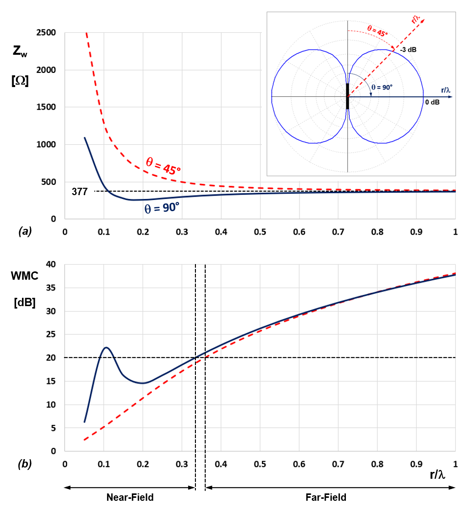
Figure 1(a) shows the absolute wave impedance as a function of distance for an elementary electric dipole and an elementary magnetic dipole, while Figure 1(b) shows the corresponding WMC. The direction along which the distance r/λ varies is perpendicular to the axis of the dipoles, where the far-field reaches its maximum value. In both cases, the 20 dB boundary is practically at r/λ = 0.33 ≈ 1/3. Additionally, we could divide the near-field region into two parts, one below the maximum at r/λ = 0.1 and one above.

Figure 2(a) displays the absolute wave impedance for an elementary electric dipole along a direction at 45° from its axis, where the power density drops 3 dB compared to its maximum value, as well as the curve obtained in the previous Fig. 1(a) along the direction at 90° from the dipole’s axis. Figure 2(b) shows the corresponding WMC. In this way, we observe the wave impedance and WMC for the directions that define the radiation maximum and the beamwidth of an elementary dipole.
We can observe that the boundary between the near-field and far-field regions moves away from the dipole when observed from a direction other than that of maximum radiation, and a transition zone opens around r/λ = 1/3.
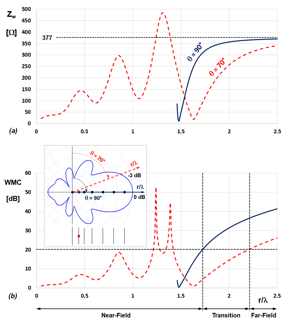
As an example of an antenna with a size of multiple wavelengths, Fig. 3 presents the results for a 7-element Yagi-Uda antenna, optimized to provide maximum front-to-back ratio. Figure 3(a) shows the absolute wave impedance in the direction of maximum radiation, perpendicular to the antenna elements, and in the direction where the maximum power density drops by half (-3 dB) and defines the edge of the beamwidth. Figure 3(b) shows the corresponding WMC curves.
In this case, the 20 dB boundary also shifts to a greater distance when the observation direction is different from the direction of maximum radiation, similar to the elementary dipole. Additionally, the transition zone between the near-field and far-field zones is approximately half a wavelength.
We can see that the wave impedance can reach very high values, so representing the WMC provides a more convenient decibel scale for comparing large and small values.
Another interesting example of a long-wavelength antenna is the axial mode helical antenna. Figure 4 shows the results for a left-handed helical antenna with a diameter of 0.3λ, a pitch of 0.22λ, and 10 turns, resulting in a total length of 2.2λ from end to end. The helix reflector, which is necessary for it to operate in axial mode (with maximum radiation along the helix axis), has a diameter of 0.95λ.
Figure 4(a) shows the wave impedance along the axis of the helix, from the base, passing through the interior of the helix until it exits. It also shows the wave impedance along a direction corresponding to the -3 dB beamwidth edge. Figure 4(b) shows the corresponding WMC results. Here, too, a displacement of the boundary between the near-field and far-field regions can be observed. We can see that as we traverse the interior of the helix along its axis, the boundary between the near and far-field zones begins at r/λ = 2.3, which is just a distance of 0.1λ above the top of the helix located at 2.2λ. This is logical since the interior of the helix behaves like a waveguide.
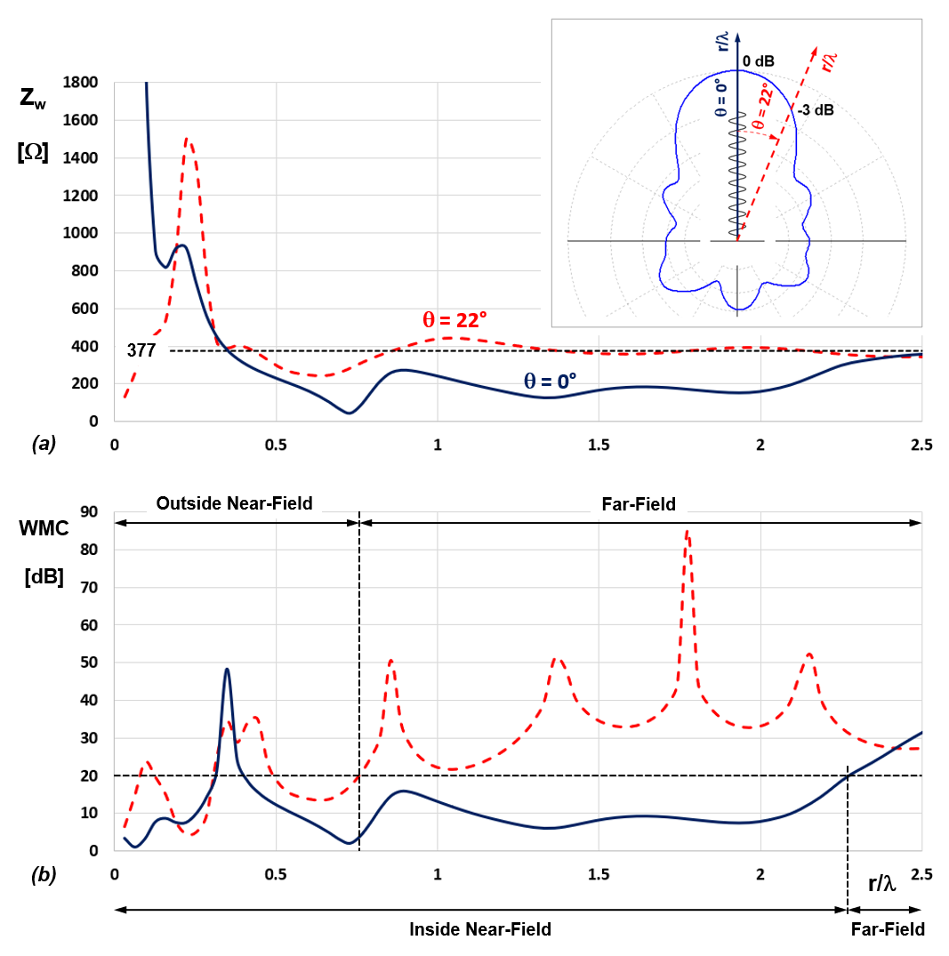
Figure 4(b) also reveals that the WMC outside the helix exhibits nearly periodic peaks due to oscillations in the absolute wave impedance around 377 Ω. While the magnitude of the wave impedance may approach 377 Ω in the near-field region, its phase will not be close to zero. To define the boundary where the far field begins, the WMC must exceed 20 dB and remain above this threshold. However, as this example illustrates, the WMC may oscillate instead of increasing monotonically.
From the examined examples, we conclude that the three-dimensional boundary between the near and far-field regions is neither spherical nor regular for antennas comparable to or larger than the wavelength. The absolute wave impedance, particularly the WMC, helps identify where the far-field region begins in each direction. The farthest boundary from this analysis can then be used as the radius of a limiting sphere, marking the start of the far-field region in all directions.
How to Obtain Wave Impedance and WMC in AN-SOF
The AN-SOF Antenna Simulator enables users to calculate the near field at a defined set of spatial points as a function of frequency. The near field calculations yield the electric ($\mathbf{E}$) and magnetic ($\mathbf{H}$) vector fields, which can be presented in Cartesian, cylindrical, or spherical coordinates.
Setting Up the Near Field Calculation
Before performing the near field computation, follow these steps:
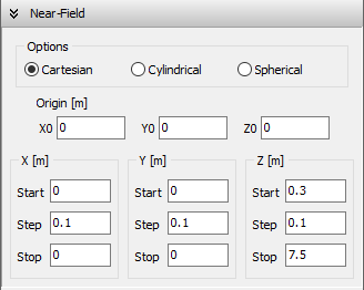
- Navigate to the Setup tab and select the Near-Field panel.
- Choose the desired coordinate system and configure the grid of points where the near field will be evaluated (refer to Fig. 5).
- Ensure the operating frequency or frequencies are set in the Frequency panel.
Once the setup is complete, execute the near field calculation by selecting Run > Run Currents and Near-Field (F12).
Accessing the Results
After the calculation is complete, go to the Results menu to access the following options:
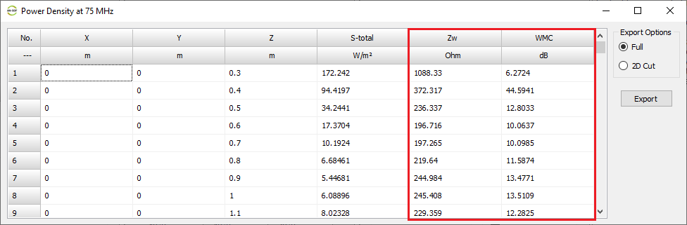
- List Power Density Pattern:
- Select a fixed frequency to view results.
- The tabulated data will include the following at the specified spatial points:
- Power density (S in W/m2)
- Absolute wave impedance (Zw in Ohms)
- Wave Matching Coefficient (WMC in dB)
- See Fig. 6 for an example.
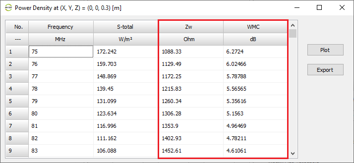
- List Power Density Spectrum:
- Select a fixed point in space to view results.
- The tabulated data will include the following as a function of frequency:
- Power density (S in W/m2)
- Absolute wave impedance (Zw in Ohms)
- Wave Matching Coefficient (WMC in dB)
- See Fig. 7 for an example.
Exporting and Analyzing the Data
Both the Power Density Pattern and Power Density Spectrum tables can be exported as CSV (Comma-Separated Values) files by clicking the Export button next to the respective table. The exported data, including Zw and WMC, can be further analyzed or plotted using spreadsheet tools such as Microsoft Excel® or Google Sheets®.
Conclusions
In this article, we introduced the concepts of absolute wave impedance and the Wave Matching Coefficient (WMC) as practical tools for defining the boundary between the near and far-field regions of an antenna. The WMC, in particular, offers improved visualization of wave propagation as a function of distance from the source antenna, using a decibel scale to highlight significant variations in wave impedance. As a general guideline, a WMC value of 20 dB serves as an effective threshold for distinguishing between the near and far-field zones.
Through examples involving elementary antennas and antennas of significant size relative to the wavelength, we observed that the 20 dB boundary lies at a distance of λ/3 for elementary antennas. However, for antennas comparable to or larger than the wavelength, the boundary takes on an irregular, non-spherical shape. In such cases, the radius of a spherical boundary separating the near-field and far-field regions is determined by the maximum distance observed in all angular directions where the WMC reaches the 20 dB threshold.
Further Reading
The traditional separation between field regions is explained in detail in section “4.4 Region Separation” of the renowned book “Antenna Theory, Analysis and Design” by Constantine A. Balanis, 4th edition, 2016, John Wiley & Sons. For a compelling analysis utilizing wave impedance, refer to “Near Field or Far Field?” by Charles Capps, EDN, Design Feature, Aug. 16, 2001, pp. 95-102. A comprehensive examination can also be found in the paper “Where Does the Far Field of an Antenna Start?” by M. Abdallah, T. Sarkar, M. Salazar-Palma, and V. Monebhurrun, published in IEEE Antennas & Propagation, Vol. 58, Issue 5, Oct. 2016, pp. 115-124.
See Also:
Technical Keywords: Wave Matching Coefficient (WMC), Absolute Wave Impedance, Near-Field/Far-Field Boundary, Transition Zone, Wave Propagation, 20 dB Threshold, Field Region Separation, Antenna Impedance Matching, Non-spherical Boundaries, Electromagnetic Wave Theory.
