Search for answers or browse our Knowledge Base.
Guides | Models | Validation | Book
Simplified Modeling of Microstrip Antennas on Ungrounded Dielectric Substrates: A Practical First-Order Approach
Discover a practical first-order method for modeling microstrip antennas on ungrounded dielectric substrates with simplicity and ease.
This article introduces a simple first-order model for estimating the input impedance and gain of planar antennas printed on ungrounded dielectric substrates with moderately high permittivity. We review existing models based on effective medium theory and introduce a novel approach that, instead of providing analytical formulas for effective permittivity, utilizes simulation software to determine antenna resonance frequencies. This approach leads to improved results compared to established effective medium formulas.
The model’s validity is confirmed through a comparison of simulation results with measured data for planar dipoles printed on FR4 substrates, which feature a standard dielectric constant of $4.5$ and a thickness of approximately $1.6 \, \mathrm{mm}$, commonly used in practical applications.
Introduction
“All models are wrong, but some are useful,” a renowned saying attributed to the British statistician George E. P. Box. This statement closely aligns with a fundamental question: to what extent can one simplify a model without compromising its ability to capture what is truly essential? How minimal can a simplified model be while still retaining its “usefulness” despite its inherent inaccuracies?
We delve into this critical question within the context of accounting for the impact of dielectric substrates on planar antennas printed on ungrounded FR4 slabs. In this article, we present a simplified method that yields results closely aligned with measurements for the input impedance and gain of planar antennas printed on FR4 dielectric substrates at microwave frequencies.
FR4 is a dielectric material with a standard relative permittivity of $4.5$, readily available in the market as flat sheets of various thicknesses, with $1.6 \, \mathrm{mm}$ being the most common. While these values may vary slightly in practice, the method we discuss is applicable to different variants of this material.
In the realm of microwave bands, antennas printed on dielectric substrates have gained immense popularity, primarily due to their practicality in supporting antenna structures measuring only a few centimeters. However, a pressing issue arises: the dielectric constant’s influence on the effective length of traces and, consequently, the resonance frequency of the antenna. To tackle this challenge, one could opt for full-wave methods, such as the Finite Element Method (FEM), which allow for the discretization of both the metallic antenna components and the dielectric substrate. Yet, this approach demands substantial computational resources, and the available software solutions often come with exorbitant costs.
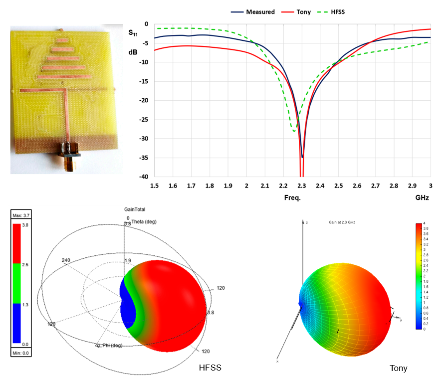
Figure 1 illustrates the precision attainable with our simplified method, which we will elucidate in the subsequent sections. It presents both simulation and measured results for a planar Yagi-Uda antenna designed for 2.4 GHz applications. The figure encompasses several components: the measured return loss,1 a photograph of the actual antenna fabricated on an FR4 epoxy dielectric, and graphs generated through HFSS software. These elements have been extracted from Ref. [1]. The red curve and radiation pattern labeled as “Tony” represent the results obtained after applying our simplified method. Here, it becomes evident that our streamlined approach accurately predicts the resonance frequency and radiation pattern of the planar Yagi-Uda antenna.
Effective Permittivity of Ungrounded Substrates
One of the most straightforward methods one might consider is replacing the dielectric substrate with an infinite medium characterized by an effective permittivity, denoted as $\varepsilon_{\mathrm{eff}}$. In this approach, the entire antenna resides within this infinite medium. Notably, this method simplifies the model by disregarding the influence of substrate edges and corners, which typically give rise to diffracted waves. The effective permittivity relies on several factors, including the dielectric constant of the substrate, the medium surrounding the substrate (commonly air, treated as free space with a relative permittivity of $1$), the substrate’s thickness, and the dimensions of the printed metal strips.
When a substrate incorporates a ground plane, typically composed of a metal plate, established theories on effective mediums offer closed analytical formulas for calculating the effective permittivity. In such cases, this is feasible because the electric field predominantly concentrates just below the strips. Utilizing techniques like conformal mapping or a transmission line model, researchers can derive closed-form expressions for the capacitance between the strips and the ground plane. Refer to Section “14.2.1 Transmission-Line Model” in Ref. [2] for further insights. However, when there is no ground plane, computing the effective permittivity becomes significantly more challenging.
In Ref. [3], researchers explored four analytical methods for estimating the effective permittivity of ungrounded substrates, ultimately concluding that two methods yield acceptable results:
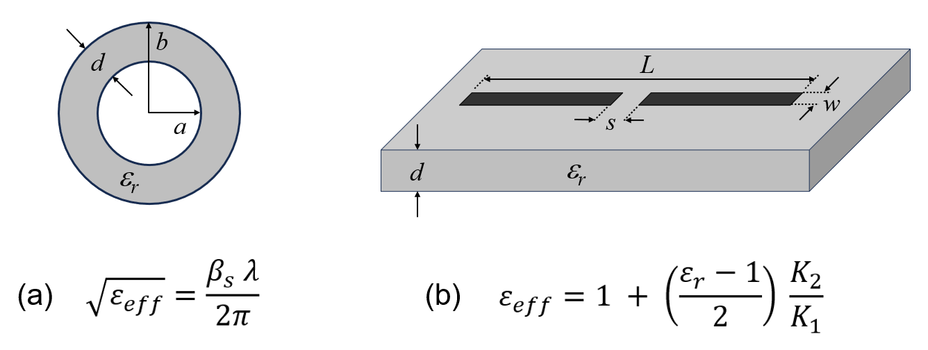
1) Insulated wire approach: This method involves considering an infinitely long circular wire covered by a dielectric sheath with the same thickness as the planar substrate. The key is to calculate the propagation constant within the sheath, denoted as $\beta_s$, as illustrated in Fig. 2(a). Consequently, the effective permittivity depends solely on the dielectric constant of the sheath and its thickness. Importantly, it does not rely on the length of the strips.
2) Coplanar strips technique: In this method, a conformal mapping transformation is utilized to calculate the effective capacitance between two parallel strips situated within the same plane. From this capacitance, the effective permittivity can be derived. This approach considers the substrate’s permittivity, its thickness, as well as the dimensions (lengths and widths) of the strips, as depicted in Fig. 2(b). The expression for $\varepsilon_{\mathrm{eff}}$ incorporates a factor denoted as $K_2/K_1$, which relies on complete elliptic integrals of the first kind:
$\displaystyle \varepsilon_{\mathrm{eff}} \,=\, 1 \,+\, \left(\frac{\varepsilon_r \,-\, 1}{2}\right) \frac{K_2}{K_1}$
Beyond the mathematical intricacies, it’s intuitive that as the substrate thickness, $d$, approaches infinity ($d \to \infty$), $K_2/K_1$ tends to $1$, yielding an effective permittivity equal to the average of the substrate and free space permittivities, $\varepsilon_{\mathrm{eff}}(d \to \infty) = (1 + \varepsilon_r)/2$. Conversely, when the thickness is zero ($d = 0$), $K_2/K_1 = 0$, and the effective permittivity equals that of free space, $\varepsilon_{\mathrm{eff}}(d = 0) = 1$. Therefore, the theory of the effective medium produces a permittivity value ranging between $1$ and $(1 + \varepsilon_r)/2$.
Methods that rely on effective permittivity offer an enticing level of simplicity. However, when applied in practice, they often result in a noticeable shift of the resonance frequency, either toward higher or lower frequencies. This phenomenon was indeed observed and documented in Ref. [3], where a comparison between simulated results and measurements for a planar dipole printed on an ungrounded FR4 substrate slab demonstrated this effect.
In the realm of microstrip antennas operating at microwave frequencies, it’s quite common for the strip width to closely align with the thickness of the FR4 substrate. In such scenarios, both the “insulated wire” and “coplanar strips” methods typically yield an effective permittivity ranging from approximately 1.5 to 1.8. This specific scenario, where strip width closely matches the substrate thickness, forms the focal point of our discussion in this article. It’s worth noting that for many practical applications, the thickness of the substrate remains a fixed parameter and is not adjustable within our simplified model.
Modeling Method Based on Resonance Frequencies
Unlike the methods described in the previous section, our proposed approach does not rely on analytical formulas to determine the effective permittivity. Instead, it is rooted in simulation techniques, and its application comprises the following steps:
1. Compute the Antenna’s Actual Resonance Frequency
The method we propose is heuristic in nature, rooted in a fundamental observation: in substrates with a permittivity high enough, when the width of the printed metal strips is close to or lower than the substrate thickness ($w \approx d$ or $w \leq d$, the electric field in very close proximity to the strips is predominantly concentrated within the dielectric substrate, rather than in free space (at microwave frequencies). This observation is crucial, as it implies that the propagation constant relevant for calculating the interaction between the strips is approximately $\beta_s = 2 \pi \sqrt{\varepsilon_r} / \lambda$, where $\varepsilon_r$ represents the relative permittivity of the substrate, and $\lambda$ denotes the wavelength in free space.
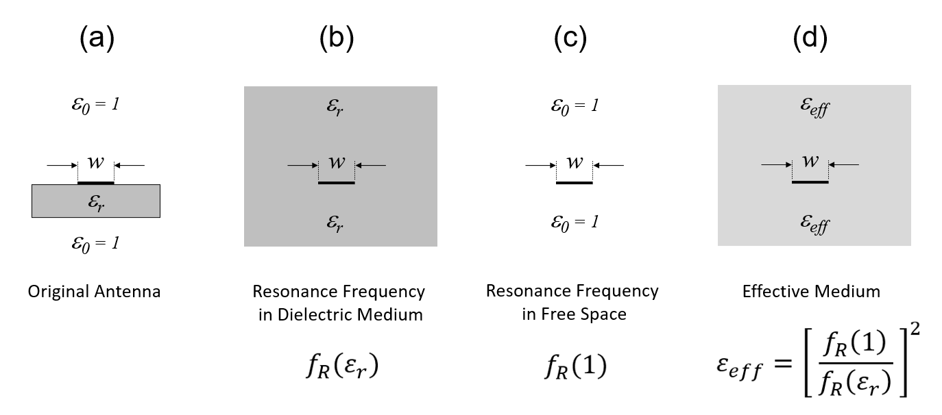
This observation has paramount significance because it suggests that the resonance frequency is primarily determined by $\varepsilon_r$ itself, rather than an effective permittivity ($\varepsilon_{\mathrm{eff}}$) as assumed in effective medium approaches. Therefore, our initial step involves calculating the resonance frequency of the antenna when it is immersed in an infinite medium with a permittivity equal to that of the substrate. This frequency, denoted as $f_R(\varepsilon_r)$, should closely align with the actual resonance frequency of the antenna on the original finite substrate, assuming a high substrate permittivity and either $w \approx d$ or $w \leq d$. Figure 3(a) illustrates the profile of the original antenna, while Fig. 3(b) depicts the antenna completely surrounded by a dielectric medium with permittivity $\varepsilon_r$, within which we must ascertain the actual resonance frequency.
2. Calculate the Effective Permittivity and Input Impedance
The radiation resistance of an antenna relies on the far-field radiation it produces, where the propagation constant corresponds to that of free space ($\beta = 2\pi/\lambda$), rather than the dielectric substrate ($\beta_s = 2 \pi \sqrt{\varepsilon_r} / \lambda$). In cases where power losses can be neglected, the input resistance of the antenna is, in fact, equal to the radiation resistance. A similar principle applies to the imaginary component of the input impedance, referred to as input reactance, which hinges on the balance between electric and magnetic energies in the vicinity of the antenna, where the dielectric substrate plays a role.
To compute the antenna’s input impedance, we must account for an effective permittivity, one that falls between the permittivity of free space and that of the substrate. Given that, from a radiation perspective, the propagation constant in free space takes precedence, our next step involves calculating the resonance frequency when the antenna exists in free space, devoid of the dielectric substrate, as depicted in Fig. 3(c). We denote this frequency as $f_R(1)$, with the “$1$” signifying the relative permittivity of free space.
It’s crucial to note that, since $f_R(1) > f_R(\varepsilon_r)$, in order to lower the resonance frequency from $f_R(1)$ to $f_R(\varepsilon_r)$, we must divide it by the square root of the effective permittivity, i.e. $f_R(1) / \sqrt{\varepsilon_{\mathrm{eff}}} = f_R(\varepsilon_r)$. Consequently, the effective permittivity is calculated as
$\displaystyle \varepsilon_{\mathrm{eff}} \,=\, \left[\frac{f_R(1)}{f_R(\varepsilon_r)}\right]^2$
This value is the permittivity that we will employ to calculate the input impedance, treating the antenna as though it is immersed in an infinite medium with a permittivity of $\varepsilon_{\mathrm{eff}}$, as illustrated in Fig. 3(d).
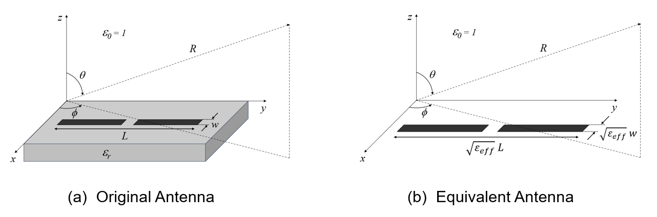
3. Rescale the Antenna to Obtain the Far Field
Our final step involves calculating the radiated far field. In the far-field zone, only the free space propagation constant, $\beta = 2\pi/\lambda$, is relevant. When viewed from a considerable distance, the impact of the substrate on the radiation pattern is essentially a dilation effect on the dimensions of the printed strips, scaled by a factor of $\sqrt{\varepsilon_{\mathrm{eff}}}$. Consequently, to create an equivalent antenna in free space without the dielectric substrate, we can increase the size of the antenna by multiplying all its dimensions, both strip lengths and widths, by the scaling factor $\sqrt{\varepsilon_{\mathrm{eff}}}$. This results in an antenna of increased size surrounded by free space,2 as illustrated in Fig. 4.
In this context, our primary focus commonly centers on the radiation pattern at the resonance frequency.
Comparisons with Measured Data
In this section, we embark on a comparison between the data generated by the method we’ve elucidated and the measurements obtained for planar dipoles printed on FR4, sourced from Ref. [3]. From this reference, we’ve also extracted results calculated using an effective permittivity corresponding to the “insulated wire” method. This approach allows us to assess the outcomes of our proposed method in comparison to measurements and another method that relies on an effective medium.
For our calculations, we employ the AN-SOF Antenna Simulator, which offers the flexibility to manipulate the permittivity of the medium surrounding the antenna and define flat strips, not restricted to wires with circular cross-sections. The first dipole in our analysis possesses dimensions of $L = 93.8 \, \mathrm{mm}$ in length and $w = 2 \, \mathrm{mm}$ in width, with the dielectric substrate being a standard FR4 characterized by a permittivity of $\varepsilon_r = 4.5$ and a thickness of $d = 1.6 \, \mathrm{mm}$. Our frequency range of interest spans from $1 \, \mathrm{GHz}$ to $1.8 \, \mathrm{GHz}$.
To initiate the process, we set the medium’s permittivity to $\varepsilon_r = 4.5$ in the Setup tab > Environment panel of AN-SOF. We then execute a frequency sweep, stepping through frequencies with a granularity of $0.01 \, \mathrm{GHz}$ to achieve three significant digits in the resonance frequency. AN-SOF operates on the Conformal Method of Moments, necessitating that the dipole be divided into segments much smaller than the wavelength. In this instance, we employ $25$ segments. At the highest frequency of $1.8 \, \mathrm{GHz}$, each segment length constitutes approximately $5\%$ of the wavelength within the dielectric medium. It’s important to note that while the wavelength at $1.8 \, \mathrm{GHz}$ in free space is $\lambda = 166.6 \, \mathrm{mm}$, the segments must be small relative to the wavelength within the dielectric medium, which is shorter than the free-space wavelength and can be calculated as $\lambda/\sqrt{\varepsilon_r} = 78.5 \, \mathrm{mm}$.
After initiating the calculation by pressing Ctrl + R and identifying the point where the imaginary part of the input impedance reaches zero, we obtain a resonance frequency of $f_R(4.5) = 1.23 \, \mathrm{GHz}$. Remarkably, with three significant figures, this result precisely aligns with the resonance frequency of the actual antenna reported by the authors of Ref. [3]. Thus, the error with this level of precision stands at $0\%$.
The next step involves calculating the resonance frequency of the antenna in free space. To do this, we return to the Setup tab > Environment panel in AN-SOF and set $\varepsilon_r = 1$. Subsequently, we rerun the frequency sweep without needing to alter the number of segments for the dipole. As the wavelength nearly doubles when $\varepsilon_r = 1$, each segment now spans approximately $2\%$ of $\lambda$. The computed resonance frequency in free space is determined to be $f_R(1) = 1.51 \, \mathrm{GHz}$. Remarkably, this result closely aligns with the reported resonance frequency of the dipole in air, which is $1.50 \, \mathrm{GHz}$, as documented in Ref. [3]. The error with this precision is merely $0.67\%$.
According to our model, the effective permittivity is now calculated as
$\displaystyle \varepsilon_{\mathrm{eff}} \,=\, \left(\frac{1.51}{1.23}\right)^2 \,=\, 1.51$
Subsequently, we set $\varepsilon_r = 1.51$ in the Environment panel within AN-SOF and initiate the input impedance calculation either by pressing Ctrl + R or through the main menu > Run > Run Currents.
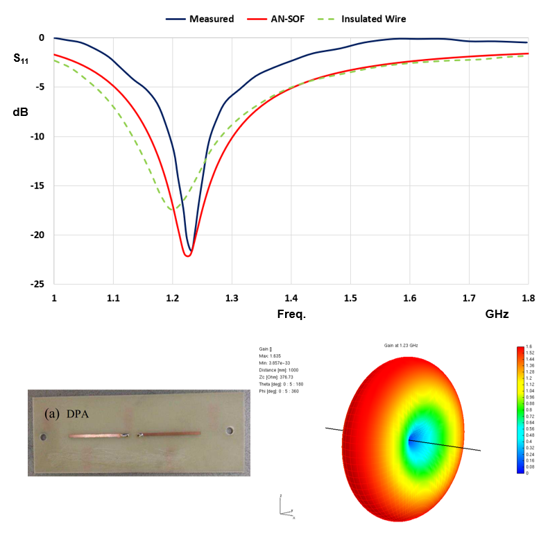
Figure 5 presents a photograph of the actual fabricated antenna, the measured return loss, and the results obtained using the insulated wire method, with all these elements extracted from Ref. [3]. Additionally, we’ve incorporated the curve obtained through AN-SOF into the graph of S11 (with a reference impedance of $50 \, \Omega$). Notably, the predictions of the resonance frequency and the mismatch at resonance (the value of S11 at $1.23 \, \mathrm{GHz}$) generated by our proposed method closely align with the measured data, surpassing the results of the insulated wire method.
Furthermore, Fig. 5 showcases the radiation pattern acquired after rescaling the dipole by multiplying its length L and width w by the factor $\sqrt{\varepsilon_{\mathrm{eff}}} = \sqrt{1.51} = 1.23$, followed by conducting calculations in free space while setting $\varepsilon_r = 1$ in the Environment panel. This analysis yields a donut-shaped radiation pattern with a maximum gain of $1.64$, which, to three significant figures, coincides with the theoretical value for a resonant dipole with a length approximately half a wavelength. We can confirm that the effective length of the dipole at $1.23 \, \mathrm{GHz}$ is $0.47 \lambda_{\mathrm{eff}}$, where
$\displaystyle \lambda_{\mathrm{eff}} \,=\, \frac{\lambda}{\sqrt{\varepsilon_{\mathrm{eff}}}}$
Now, let’s consider a second dipole, which possesses a length of $L = 72.5 \, \mathrm{mm}$ and the same width as the previous one, $w = 2 \, \mathrm{mm}$. This second dipole has been obtained by rescaling the first one in order to achieve a resonance frequency of $1.5 \, \mathrm{GHz}$, although in the measurements, as reported by the authors of Ref. [3], a value of $1.49 \, \mathrm{GHz}$ was obtained. By following the same procedure as the one outlined earlier, we determined $f_R(4.5) = 1.50 \, \mathrm{GHz}$ and $f_R(1) = 1.94 \, \mathrm{GHz}$ for the scaled dipole. Consequently, the effective permittivity for this case is calculated as
$\displaystyle \varepsilon_{\mathrm{eff}} \,=\, \left(\frac{1.94}{1.50}\right)^2 \,=\, 1.67$
It’s worth noting that to obtain the resonance frequencies for this dipole, we had to employ $51$ segments. In each instance, an analysis of result convergence based on the number of segments is imperative.
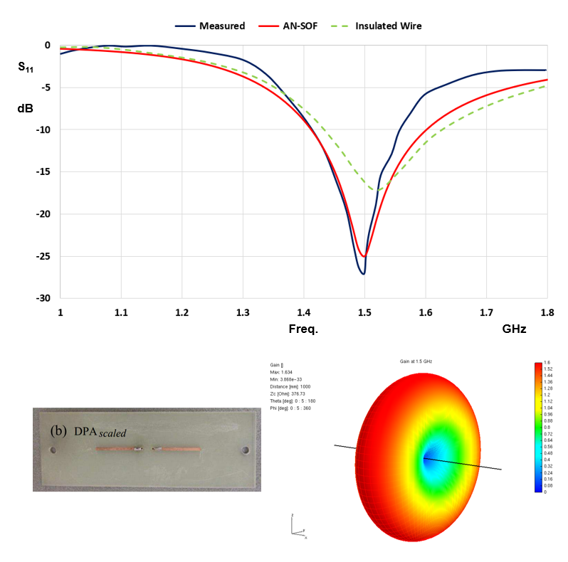
Figure 6 presents the results for the scaled dipole. We include a photograph of the dipole, the measured S11 curve, and the curve calculated using the insulated wire model, all sourced from Ref. [3]. Additionally, we’ve superimposed the curve obtained by AN-SOF onto the S11 graph. It’s evident that the fit with the measured data is exceptionally satisfactory, surpassing the precision achieved through other methods. The radiation pattern is also depicted, boasting a gain of $1.64$, aligning with our expectations.
Conclusions
Recalling the introductory phrase of this article, “All models are wrong, but some are useful,” we have introduced a model here that indeed falls into the category of being “wrong.” It neglects the diffraction of waves at the edges and corners of the dielectric substrate and does not account for substrate thickness, necessitating sufficiently high permittivity and strip widths comparable to or lower than the substrate thickness.
However, it is an exceedingly simple model, arguably one of the simplest conceivable, and it yields valuable results that closely align with measured data. This model leverages the capabilities of simulation software tailored to wire antennas, such as AN-SOF, offering a cost-effective solution for designing microstrip antennas on ungrounded dielectric substrates.
In summary, the construction of the model involves the following steps:
- Determine the antenna’s actual resonance frequency by assuming it is submerged in an infinite medium with the same permittivity as the dielectric substrate, denoted as $f_R(\varepsilon_r)$.
- Determine the antenna’s resonance frequency in free space, in the absence of the substrate, denoted as $f_R(1)$.
- Calculate the input impedance, from which the return loss (S11) can be derived, by simulating the antenna in an infinite medium with an effective permittivity of $\varepsilon_{\mathrm{eff}} = [f_R(1) / f_R(\varepsilon_r)]^2$. The radiation pattern is obtained by rescaling the antenna in free space, multiplying its dimensions by the factor $\sqrt{\varepsilon_{\mathrm{eff}}}$.
The model we’ve introduced considers antenna dimensions, including the lengths and widths of the printed strips, to determine effective permittivity through the resonance frequencies $f_R(\varepsilon_r)$ and $f_R(1)$. Therefore, the influence of antenna geometry and its dimensions is inherently incorporated into our effective permittivity calculation. In contrast, effective media methods frequently encounter challenges when dealing with complex antenna geometries, and analytical formulas are typically limited to simpler cases, such as the planar dipole. This distinction underscores the accuracy of our method, particularly in determining resonance frequencies for microstrip antennas.
See Also:
References
[1] “High Gain Improved Planar Yagi Uda Antenna for 2.4 GHz Applications and Its Influence on Human Tissues,” by Claudia Constantinescu et al., Appl. Sci. 2023, 13, 6678.
[2] “Antenna Theory Analysis and Design” by Constantine A. Balanis, 4th Edition, Wiley 2016.
[3] “A Robust Method of Calculating the Effective Length of a Conductive Strip on an Ungrounded Dielectric Substrate” by M. Kanesan, D. V. Thiel, and S. O’Keefe, Progress In Electromagnetics Research M, Vol. 35, 57–66, 2014.
Footnotes
- In microstrip antennas, it is customary to present the reflection coefficient at the feed port, denoted as S11, rather than the input impedance, as S11 is the more frequently measured parameter. In technical terms, S11 expressed in decibels is often referred to as “return loss.” However, it’s important to clarify that the formal definition of return loss is the negative of S11 in decibels.
↩︎ - Instead of rescaling the antenna dimensions and reiterating the calculations for obtaining the radiation pattern, a simpler approach is to keep the dimensions constant and adjust the frequency by multiplying it by $\sqrt{\varepsilon_{\mathrm{eff}}}$. This method allows us to leverage the calculations already performed in free space to determine the resonance frequency $f_R(1)$.
↩︎
