Search for answers or browse our Knowledge Base.
Guides | Models | Validation | Book
Modeling a Center-Fed Cylindrical Antenna with AN-SOF
Learn how to simulate a center-fed cylindrical antenna using AN-SOF software. This step-by-step guide covers setup, geometry creation, simulation, and result analysis. Understand dipole characteristics through practical examples.
Introduction: Center-Fed Cylindrical Antenna Simulation
The center-fed cylindrical antenna serves as a fundamental example for simulation. Essentially a straight wire with a central excitation, it transitions into a half-wave dipole when its length aligns with half the wavelength of the operating frequency. The following steps outline the simulation process using AN-SOF.
Step 1: Configuring the Simulation Environment
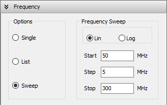
To initiate, navigate to Tools > Preferences within the main menu to establish appropriate units for frequency (MHz) and length (m). Subsequently, access the Setup tab. Within the Frequency panel, select Sweep and configure the Frequency Sweep parameters as depicted in Fig. 1. The calculations will be performed at the frequencies: 50, 55, …, 295, 300 MHz. Ensure that None (free space) is chosen in the Environment panel‘s Ground Plane box and Discrete Sources is selected under the Excitation panel.
Step 2: Creating the Antenna Geometry
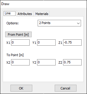
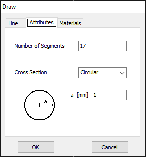
To initiate the antenna geometry creation, right-click within the workspace and select Line from the ensuing pop-up menu. The ‘Line’ dialog box will appear. Populate the Line and Attributes pages as outlined in Figs. 2 and 3 to generate a straight wire comprising 17 segments and a 1 mm radius within the workspace. The wire will be drawn starting from point (0,0,-0.75) [m] and ending at point (0,0,0.75) [m], aligning with the z-axis and spanning a length of 1.5 m, equivalent to a half-wavelength at 100 MHz. Press F7 to visualize the primary axes.
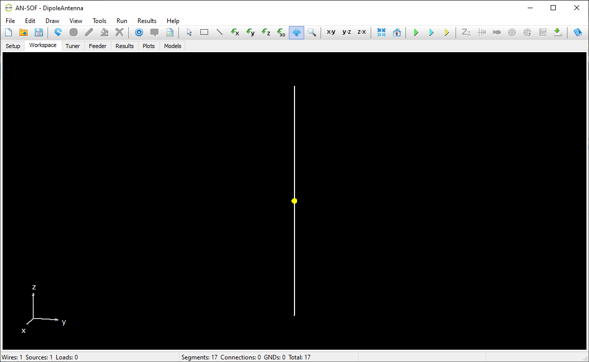
Subsequently, right-click on the wire and choose Source/Load/TL from the context menu. Following the procedure detailed in “Adding Sources,” introduce a voltage source at the wire’s center (segment 9). Set the source voltage to 1 (0°) V. The resulting center-fed cylindrical antenna in the AN-SOF’s workspace is represented in Fig. 4.
Step 3: Simulation Execution and Result Analysis
To initiate the simulation process, click the Run Currents and Far-Field (F11) button on the toolbar. Upon completion, right-click on the wire and select Plot Currents from the context menu, specifying the desired frequency. The resulting current distribution along the wire is graphically represented in Fig. 5. To access additional parameters of interest, refer to the procedures outlined in “Displaying Results.”
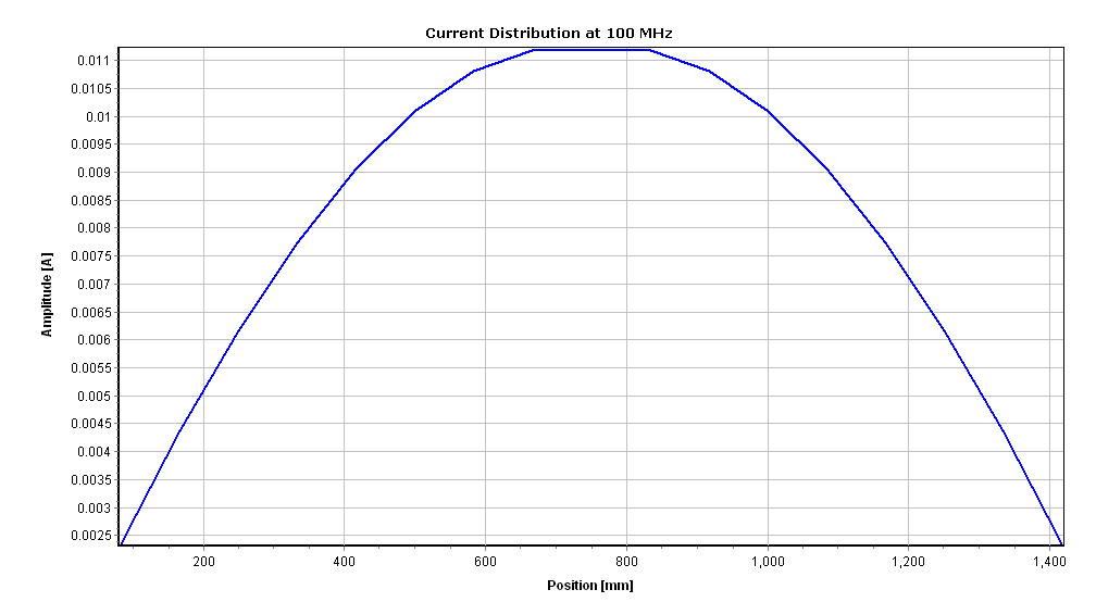
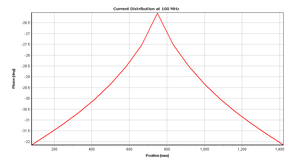
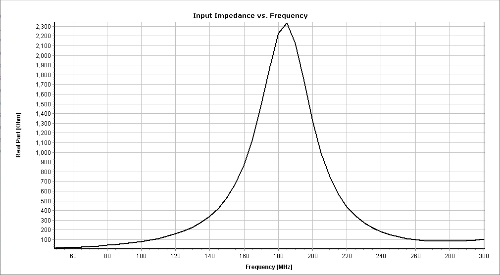
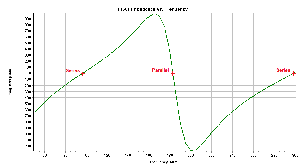
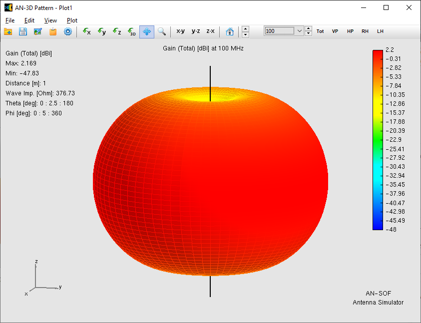
As an illustrative example, Figures 5, 6, and 7 depict the current distribution at 100 MHz (amplitude in Fig. 5(a) and phase in Fig. 5(b)), input impedance versus frequency (real part in Fig. 6(a) and imaginary part in Fig. 6(b)), and gain pattern in dBi (Fig. 7) at 100 MHz.
Given that the antenna length (1.5 m) equals half a wavelength at 100 MHz, the current distribution in amplitude approximates a half-cycle sine function, aligning with the expected behavior of a half-wave dipole. A slight decrease in the amplitude and a sharp increase in the phase can be seen at the antenna center, due to the presence of the voltage source just there. The presence of the voltage source at the center disrupts the continuity of the current’s slope (derivative) at that point, while the current itself remains continuous.
If we look closely at Figure 6(b), which shows the input reactance (imaginary part of the input impedance), we can see that the curve crosses zero just before 100 MHz, with a positive slope (series resonance), then crosses zero again just above 180 MHz, with a negative slope (parallel resonance), and then crosses zero again just below 300 MHz with a positive slope (series resonance). These three points where the reactance vanishes correspond to when the physical length of the dipole approaches: λ/2, λ, and 3λ/2. The resonances do not occur exactly at integer values of half wavelength because the thickness of the dipole is not infinitesimal. In Figure 6(a) we can see that the input resistance is maximum at the frequency that corresponds to the parallel resonance. All these are the expected and classical behaviors of a dipole of finite thickness.
Regarding the gain pattern in Fig. 7, it is donut-shaped as expected for a half-wave dipole, with a maximum of 2.17 dBi. We should remember that the theoretical peak gain of an infinitesimally thin half-wave dipole in free space with a perfect sinusoidal current distribution is 2.15 dBi (corresponding to a numerical gain of 1.64). The obtained gain in AN-SOF is 0.02 dBi higher than the theoretical value due to the finite radius of the cross-section of the dipole.
Conclusion
This tutorial provided a step-by-step guide to simulating a center-fed cylindrical antenna using AN-SOF Antenna Simulator. By following the outlined procedures, users can efficiently model this fundamental antenna type and analyze its key characteristics.
The simulated results align with the expected behavior of a half-wave dipole, demonstrating the software’s accuracy in predicting current distribution, input impedance, gain, and radiation patterns. The influence of the antenna’s finite thickness on the resonance frequencies and gain was also highlighted.
This example serves as a foundation for more complex antenna designs. By understanding the simulation process for this simple geometry, users can apply similar principles to model and analyze a wide range of antenna structures.
