Navigating the Numerical Landscape: Choosing the Right Antenna Simulation Method

Created OnApril 7, 2024

Updated OnMay 14, 2024

By:Tony Golden

Here we present an overview of various numerical techniques used in Computational Electromagnetics (CEM), with a special focus on antenna simulation methods. We conceptually describe the following methods:

Finite Difference Time Domain (FDTD)
Finite Element Method (FEM)
Method of Moments (MoM)
Conformal Method of Moments (CMoM)
Fast Multipole Method (FMM)
Multilevel Fast Multipole Method (MLFMM)
Finite Volume Time Domain (FVTD)
Geometrical Optics (GO)
Geometrical Theory of Diffraction (GTD)
Uniform Theory of Diffraction (UTD)
Physical Optics (PO)
Physical Theory of Diffraction (PTD)
Domain Decomposition Method (DDM)

Introduction

The landscape of antenna simulation techniques has evolved significantly in recent years. While sophisticated commercial software packages offer a variety of solvers and often automate the method selection process, understanding the underlying principles of each approach remains crucial for interpreting results accurately, particularly when discrepancies arise between simulations and theoretical or experimental data.

This article delves into the various numerical methods employed in Computational Electromagnetics (CEM) and provides guidelines for selecting the most suitable technique for your specific antenna project.

Numerical methods used in CEM can be broadly classified into three main categories:

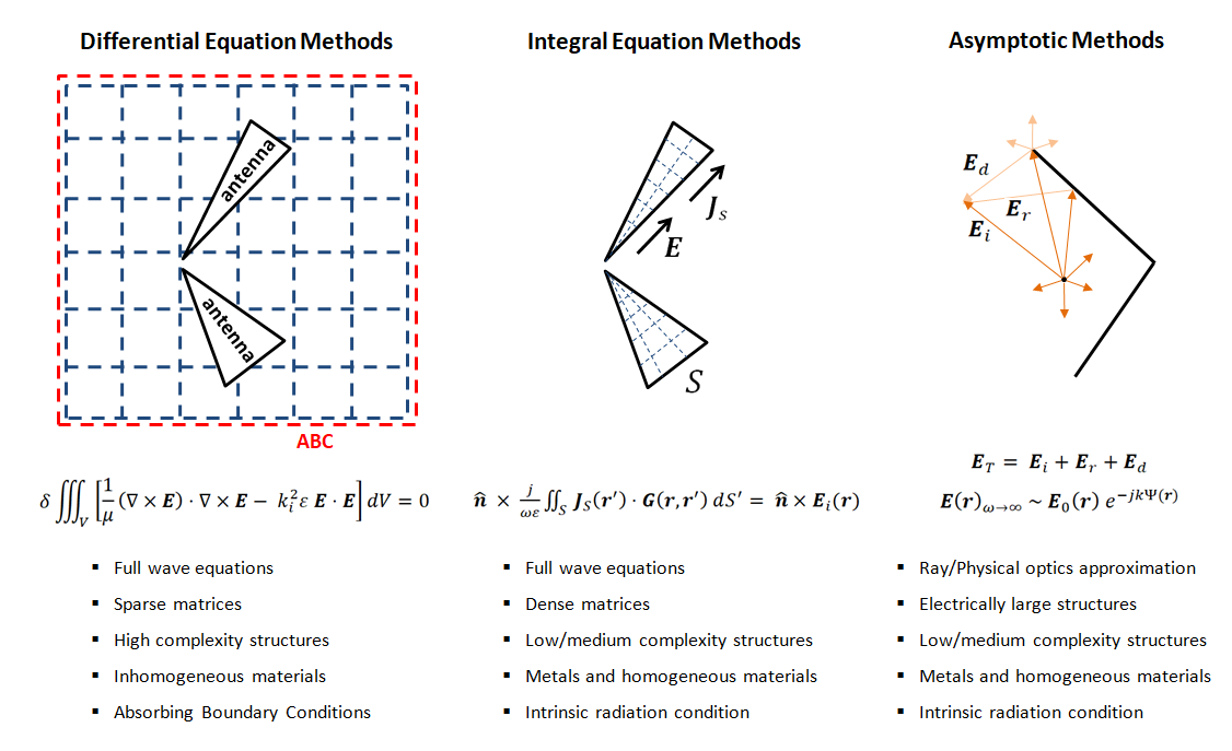
Differential Equation Methods

Differential equation methods attack the problem of antenna simulation directly by discretizing Maxwell’s equations in their partial differential equation (PDE) form. This process involves converting partial derivatives into finite difference equations, where ratios of finite subtractions approximate the actual derivatives. For example, the derivative of a function f at a point x₀ can be approximated by:

df/dx ≈ [f(x₀ + h) – f(x₀ – h)] / (2h)

where h is a sufficiently small value.

In the time domain, a time sampling scheme is also defined. This allows capturing the system’s response to a given excitation across a wide bandwidth by computing its response to the impulse function only once. This forms the basis of the Finite Difference Time Domain (FDTD) method.

In contrast, the frequency domain approach eliminates the time variable t after factoring out the common complex exponential factor exp(jωt) (where ω is the angular frequency). However, this requires repeated calculations for each frequency within the desired bandwidth, leading to increased computational cost.

The Finite Element Method (FEM) takes a different approach by deriving a functional from a volume integral of the vector wave equation. Minimizing this functional and discretizing the space into small elements, similar to FDTD, yields a finite set of linear equations for the electromagnetic field. When written in matrix form, these equations exhibit sparsity due to the localized interactions between elements. This sparsity translates to lower memory requirements for storing and solving the system compared to dense systems of similar size.

Here are some key points to note:

✅ Differential equation methods solve Maxwell’s equations directly or using a variational principle based on the vector wave equation.

✅ FDTD operates in the time domain, while FEM can work in both time and frequency domains.

✅ FEM and FDTD result in sparse matrices, reducing memory requirements.

✅ Both methods discretize the problem space into small elements.

FDTD requires only one calculation for the impulse response, while FEM requires calculations for each frequency of interest.

Differential equation methods like FDTD and FEM require special considerations when applied to antenna simulations due to the “open problem” nature of antennas. This means that boundary conditions need to be satisfied not only in the vicinity of the antenna but also at infinity, representing the radiation or Fraunhofer boundary condition.

Since it’s impossible to discretize towards infinity, both FDTD and FEM require a finite-sized box surrounding the antenna. This box needs to be equipped with Absorbing Boundary Conditions (ABC) on its faces to absorb outgoing waves and prevent reflections that can contaminate the solution.

This limitation restricts the applicability of differential equation methods to antennas that are not too electrically large. Therefore, they are not the optimal choice for simulating:

✅ Reflector antennas: These antennas typically have large reflective surfaces, making them electrically large and unsuitable for FDTD or FEM analysis.

✅ Aperture antennas: Similar to reflector antennas, these antennas also have large apertures and are not well-suited for these methods.

✅ Large arrays of wire antennas: Arrays with a large number of elements can become computationally expensive to simulate using differential equation methods.

However, these methods are well-suited for certain types of antennas:

✅ Antennas composed of inhomogeneous materials: FDTD and FEM can effectively handle antennas with complex material properties, making them ideal for simulating antennas with composite materials or dielectric substrates.

✅ Antennas with complex geometries: These methods can accurately model antennas with intricate geometries, including microstrip patch antennas with multiple layers and traces.

✅ Antennas requiring multiple boundary conditions: Differential equation methods can efficiently handle situations where different boundary conditions must be satisfied in various regions surrounding the antenna.

Therefore, while FDTD and FEM have limitations for electrically large antennas, they remain valuable tools for simulating antennas with complex materials, geometries, and boundary conditions. Their ability to accurately model microscopic details makes them particularly well-suited for microstrip patch antennas and other intricate planar antenna designs.

Integral Equation Methods

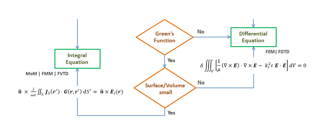
Integral equation methods, also known as Boundary Element Methods (BEM), offer an alternative approach to antenna simulation. These methods rely on a fundamental solution to Maxwell’s equations, represented by the Green’s function G. This function describes the system’s response to a spatial impulse function.

The core principle of integral equation methods lies in expressing the electromagnetic field as an integral of G-weighted equivalent currents flowing on the antenna’s boundaries. By leveraging this insight, an integral equation is derived based on the boundary conditions at the antenna surface and the interfaces between homogeneous regions.

To solve this integral equation, the unknown surface current distribution J_s is expanded into a series of basis functions with unknown coefficients. Projecting this current expansion onto a set of weighting functions leads to a matrix equation, forming the basis of the widely used Method of Moments (MoM).

A key advantage of integral equation methods lies in their reduced dimensionality. Only the antenna’s boundaries need to be discretized, eliminating the need for volume integrals as in FDTD and FEM. This simplifies the problem and reduces computational requirements.

Moreover, integral equations enable direct calculation of the radiated field from the antenna’s vicinity towards infinity. This is achieved through direct integration using the Green’s function, avoiding the space discretization and ABCs required in FDTD and FEM.

However, this benefit comes at a cost. Unlike the sparse matrices found in FDTD and FEM, the matrices in MoM are dense. This can lead to increased memory requirements and computational complexity.

Here are some key takeaways:

✅ Integral equation methods leverage the Green’s function to express the electromagnetic field.

✅ The Method of Moments (MoM) is a widely used integral equation method for antenna simulation.

✅ Integral equation methods require only boundary discretization, reducing the problem’s dimensionality.

✅ Direct calculation of radiated fields towards infinity is possible without ABC.

✅ Compared to sparse matrices of the same size in FDTD and FEM, dense matrices in MoM require more memory and computational resources.

While they come with their own set of challenges, integral equation methods offer several advantages for simulating certain types of antennas. Their reduced dimensionality and ability to handle unbounded problems make them particularly suitable for large electrically-sized antennas and structures with complex geometries.

Integral equation methods, particularly the MoM, offer significant advantages for simulating a wide range of antenna types. This is due in part to the availability of closed-form Green’s functions for various scenarios:

✅ Free space: MoM can readily handle antennas in free space, making it suitable for simulating radio antennas, satellite antennas, and other free-space radiating structures.

✅ Ground planes: Closed-form Green’s functions exist for antennas positioned over or below imperfect ground planes, allowing for accurate simulations of antennas mounted on vehicles, ships, and other grounded platforms.

✅ Stratified media: MoM can effectively analyze antennas operating in stratified media, such as antennas embedded within the earth’s surface or antennas operating in the presence of layers of dielectric materials.

✅ Periodic materials: Antennas in the vicinity of periodic materials, such as metamaterials or gratings, can also be accurately simulated using MoM with the appropriate Green’s functions.

Integral equation methods are well-suited for simulating metallic surfaces or wires. The MoM is particularly powerful for modeling wire antennas and metallic structures that can be considered perfect electrical conductors (PEC) or have very high conductivity (σ → ∞). Ohmic losses can be readily incorporated into the models using analytical formulas for skin depth.

Traditionally, the MoM is implemented by discretizing metal surfaces and wires using linear elements, typically planar triangular patches (referred to as RWG basis functions) and thin straight cylinders for wire segments. In contrast, conformal methods employ patches and segments with curvature, adapting to the shape of the boundary they represent. This approach addresses the stair-casing error inherent in linear element implementations. One such method is the Conformal Method of Moments (CMoM), which, in its initial applications, successfully eliminated discretization errors in the geometry of curvilinear loops. Furthermore, conformal extensions exist for various numerical techniques including BEM, FEM, and FDTD.

This broad range of applicability makes MoM a versatile tool for simulating diverse antenna configurations.

For electrically large structures, the MoM can be further optimized by employing the Fast Multipole Method (FMM). FMM works by dividing the problem domain into smaller subdomains and approximating the interactions between them using the multipole expansions. This significantly reduces the computational cost compared to traditional methods, making it particularly valuable for analyzing large antennas.

The Multilevel Fast Multipole Method (MLFMM) builds upon the existing FMM, offering even greater efficiency for analyzing large and complex electromagnetic problems. Here’s the gist:

FMM: Divides the domain into subdomains, approximates interactions between them, and reduces computational cost.

MLFMM: Takes FMM a step further by recursively subdividing subdomains into smaller ones, creating a hierarchical octree structure. This further reduces the complexity of interaction calculations and boosts its efficiency for even larger problems.

Advantages of MLFMM:

✅ Dramatically scales down memory and computational requirements compared to FMM, especially for electrically large structures.

✅ Maintains high accuracy even with complex geometries.

✅ Offers faster solution times for iterative solvers.

Moreover, MLFMM is well suited for parallelization. Its hierarchical structure facilitates efficient workload distribution across multiple processors, leading to significant acceleration in computation time, particularly for large-scale and complex problems like analyzing massive antenna arrays.

While MoM and FMM operate in the frequency domain, other integral equation methods like the Finite Volume Time Domain (FVTD) offer time-domain solutions. Inspired by computational fluid dynamics, FVTD provides conformal treatment of boundaries, making it suitable for analyzing antennas with complex geometries and intricate details.

Historically, the discretization of volumes and surfaces posed a significant challenge in numerical methods. However, the advent of powerful Computer-Aided Design (CAD) tools has revolutionized meshing capabilities. Today, automated meshing algorithms exist not only for CEM applications but also for various branches of Computational Physics, significantly simplifying the modeling process.

Asymptotic Methods

Asymptotic methods, also known as high-frequency methods, offer efficient solutions for simulating electrically large antennas, typically exceeding two orders of magnitude of a wavelength in size. In such cases, traditional full-wave methods like MoM and FEM would result in impractically large matrices, making them impractical for analysis.

Asymptotic methods exploit the high-frequency limiting case of Maxwell’s equations (ω → ∞) for these large structures. In this limit, electromagnetic fields behave like rays emanating from sources and interacting with the boundaries between media, where they undergo reflection, refraction, and transmission.

Geometrical Optics (GO) forms the core of this approach, describing the propagation of these rays, which can have plane, spherical, or cylindrical wavefronts. Additionally, diffracted rays appear due to scattering at edges and corners, addressed by the Geometrical Theory of Diffraction (GTD).

However, GTD calculations can exhibit infinite fields in certain ray directions, known as “caustics.” To address this issue, the Uniform Theory of Diffraction (UTD) provides a smooth solution, resolving these singularities.

Analogous to GO, Physical Optics (PO) utilizes equivalent currents flowing on metallic surfaces or boundaries between different refractive indexes to express the fields via surface integrals. This, in turn, leads to the Physical Theory of Diffraction (PTD), which employs equivalent contour currents to account for diffracted fields from edges and corners.

PTD offers the advantage of smooth solutions without requiring a uniform theory like UTD. However, it necessitates the evaluation of surface or contour integrals, making it computationally heavier than the simpler UTD approach.

Asymptotic methods represent the most efficient way to analyze electrically large antennas. They also offer significant flexibility for hybridization with other methods, particularly integral equation methods like MoM. This is especially advantageous for antennas where a smaller part interacts with a much larger structure, such as reflector, aperture, and lens antennas.

Here are some key takeaways:

✅ Asymptotic methods are highly efficient for electrically large antennas.

✅ GO and PO provide the foundation for describing ray propagation and equivalent currents, respectively.

✅ GTD and PTD address diffracted fields, with UTD offering a smooth solution for GTD singularities.

✅ Asymptotic methods are ideal for standalone analysis of large antennas and for hybridization with other methods in complex antenna configurations.

A Guide to Selecting the Best Antenna Simulation Method

We’ve explored various numerical methods for antenna simulation, each with its strengths and limitations. The best method for your project depends on various factors, including:

1. Antenna Size:

✅ Electrically large antennas (100+ wavelengths): Asymptotic methods like GO or PO are efficient and can be combined with other methods for hybrid solutions.

✅ Small to medium antennas (up to ~100 wavelengths): Integral equation methods like MoM are well-suited for antennas with metallic surfaces or wires and high conductivity.

✅ Complex materials: Differential equation methods like FDTD or FEM are preferred when Green’s functions are unknown or material complexity is high.

2. Material Complexity:

✅ Metallic surfaces or wires: Integral equation methods, particularly the MoM, are highly effective and represent the most suitable choice.

✅ Homogeneous dielectrics or magnetics: MoM can be used if Green’s functions are known and the number of surface elements is manageable.

✅ Unknown Green’s functions or high material complexity: Differential equation methods are preferred.

3. Hybridization:

✅ Fuzzy boundaries between categories: When clear-cut decisions are difficult, hybrid methods combining different approaches offer efficient solutions.

Here’s a visual decision diagram to help you choose the best method:

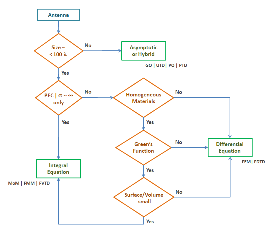
In the decision diagram above, variables such as antenna size in wavelengths (λ), medium conductivity (σ), and the presence of a Perfect Electrically Conducting medium (PEC) are considered as the main inputs for selecting an optimum antenna simulation method. The “Surface/Volume” ratio represents the number of surface elements to volume elements required to discretize the problem domain and achieve a specified accuracy. For small ratios, integral equation methods are preferred.

Remember, this is a general guide. The specific choice depends on your specific antenna project and its unique characteristics.

A Grand Innovation: The Domain Decomposition Method (DDM)

We would be remiss not to mention the Domain Decomposition Method (DDM), which defies easy categorization within the previously discussed methods. While possessing characteristics of a hybrid approach, DDM stands on its own as a powerful numerical technique for tackling complex large-scale problems.

DDM operates by dividing the computational domain into smaller, more manageable subdomains. Each subdomain is then solved independently, with the final solution obtained by combining these individual solutions through carefully chosen interface (boundary) conditions. This approach offers several compelling advantages:

Memory Efficiency: Solving the entire domain at once can quickly exhaust available memory resources. DDM circumvents this issue by focusing on smaller subdomains, significantly reducing the memory footprint. This allows us to handle large and intricate structures with relative ease.

Parallel Computations: Each independent subdomain solution opens the door for efficient parallelization. Utilizing multicore or distributed computing systems allows for significant computational speedups compared to solving the entire domain sequentially.

Flexibility: DDM boasts compatibility with various numerical methods, including FEM, BEM, and FDTD. This flexibility empowers us to choose the most suitable method for each subdomain based on its unique characteristics, leading to optimal results.

Efficient Analysis of Complex Structures: DDM excels in analyzing structures with diverse material properties and intricate geometries. By dividing the structure into subdomains with specific properties, DDM simplifies the analysis process and allows for tailoring the chosen numerical method to each individual region.

Here are some specific applications of DDM in CEM:

✅ Large antenna arrays: DDM can efficiently analyze the interaction between elements in large antenna arrays, improving the design and performance optimization.

✅ Metamaterials: DDM allows for efficient modeling of metamaterials with complex geometries and material properties, leading to better understanding and design of these advanced materials.

✅ Antenna systems on platforms: DDM can analyze the interaction of antennas mounted on large platforms like aircraft or ships, ensuring optimal performance and minimizing interference.

✅ Radar Cross Section (RCS) computation: DDM can efficiently compute the RCS of complex composite targets, providing valuable information for radar design and stealth technology.

With its unique capabilities and wide range of applications, DDM has earned its place as a groundbreaking innovation in the field of CEM.