Electric Field Integral Equation

The current distribution on metallic surfaces with ideal conductivity can be found by solving an Electric Field Integral Equation (EFIE) expressed in the frequency domain:

where:

E_i: Incident Electric Field on the surface S.

n: unit vector at point r on the surface S.

k: wave number.

J: unknown electric current density flowing on the surface.

G: Green’s function, which in free space is given by:

The EFIE is an expression of a boundary condition on the surface, namely zero tangential electric field. When we are dealing with a wire structure, the EFIE reduces to:

where T is the tangential unit vector describing the wire contour along its axis, I(s) is the unknown electric current on the wire, and K(s,s‘) is the integral equation Kernel defined as:

The EFIE is averaged about the wire circumference, resulting in the EFIE (3) with the Kernel (4). The current distribution I(s) is then the average value of the current density J in the axial direction; the current in the transversal direction is neglected. This is a good assumption provided that the wire radius is small with respect to the wavelength.

The wire axis is defined by its parametric equations that can be written in the compact form:

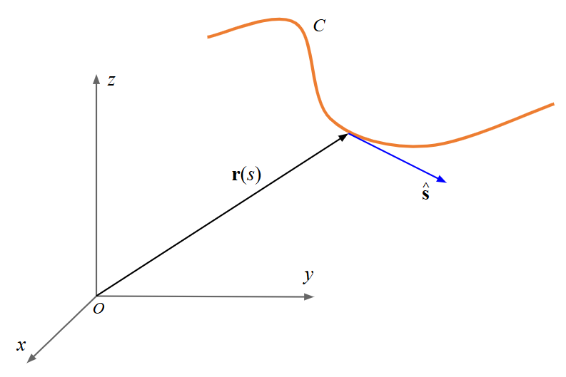
which points from the origin to any point on the wire, Fig. 1. The parameter s varies over a real interval. The tangent unit vector can be obtained from the first derivative of (5):

This parametric description is the key for the accurate modeling of wire structures. A straight wire approximation to the geometry produces a loss of geometrical information that can never be completely restored. However, this information is not lost if a parametric representation is used to describe the wire locus. It is also possible to improve on the straight wire approximation by using quadratic segments to model the geometry.

Thus, the definition of a wire must include its parametric description and its first derivative if an exact representation of the geometry is required, as shown in Fig. 1.

The Kernel (4) can be approximated by the following generalized thin-wire approximation:

where a is the wire radius.

When the observation point r(s) and the source point r(s‘) are both in the same straight wire, the distance R reduces to the usual thin-wire approximation:

Thus, the EFIE and its Kernel are also valid for straight wires.

It is well known that the thin-wire approximation produces numerical oscillations in the computed current distribution near wire ends and near the position of discrete sources when wire segments are relatively thick. To avoid this undesired behavior and obtain the maximum accuracy, the exact Kernel in (4) is used in AN-SOF by default instead of the thin-wire approximation in (7). A closed-form expression for the exact Kernel has been found so its use practically does not compromise the speed of the simulation. However, an extended thin-wire Kernel has been calculated that also avoids the current distribution inaccuracies for a thin-wire ratio (wire diameter/segment length) < 3, which is far better than the thin-wire ratio < 1 that must be used when the standard thin-wire approximation is used.

In the Settings panel > of the Setup tabsheet check the Exact Kernel option to use the exact Kernel in (4). Uncheck this option to use the extended thin-wire Kernel.

The existence of a PEC ground plane is modeled in AN-SOF by means of image currents. This method can be easily implemented by adding an image term to the Green’s function, resulting in an additional term for the Kernel.