Search for answers or browse our Knowledge Base.
Guides | Models | Validation | Book
Plotting 2D Far-Field Patterns
Rectangular Plots
The radiation pattern can be visualized as a 2D rectangular plot by navigating to Results > Plot Far-Field Pattern > 2D Rectangular Plot from the main menu. This action opens the Radiation Pattern Cut dialog box (Fig. 1), which offers two primary cut types:
- Conical Plots: Generated with a fixed $\theta$ (Theta, zenith) and variable $\phi$ (Phi, azimuth).
- Vertical Plots: Created with a fixed $\phi$ (Phi, azimuth) and variable $\theta$ (Theta, zenith).
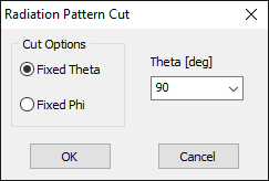
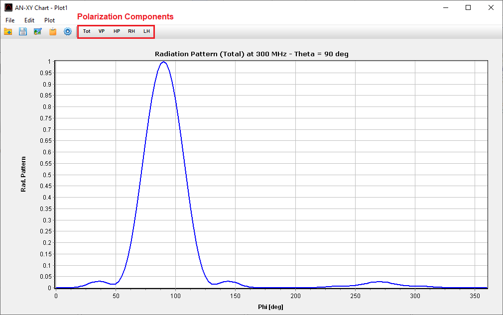
Upon selecting a cut and clicking OK, the AN-XY Chart application (Fig. 2) is launched. The pattern is plotted against Phi for conical cuts or against Theta for vertical cuts.
Parameter Visualization and Polarization
Within the AN-XY Chart application, the Plot menu allows you to graph a comprehensive suite of parameters, including:
- Metrics: Power Density, Directivity, Gain, E-field, and Axial Ratio.
- Units: Data can be represented in linear units or decibels (e.g., dBi for directivity and gain).
- Polarization Decomposition: Metrics can be decomposed into:
- Linear Components: Theta (VP: Vertically Polarized) and Phi (HP: Horizontally Polarized).
- Circular Components: Right (RHCP) and Left (LHCP).
The toolbar provides rapid-access buttons (Tot, VP, HP, RH, LH) to switch between the total field and its polarized components, facilitating a detailed analysis of the antenna’s polarization purity.
Receiving and Scattering Modes (RCS)
When using plane wave excitation, where the antenna is in receiving mode or a metallic structure is scattering waves, the software automatically plots the Radar Cross Section (RCS) instead of directivity or gain. This scattered field pattern is observed in the far-field region, where the scattered field amplitude decays at a rate of $1/r$ and the power density follows the inverse square law ($1/r^2$).
The Axial Ratio
The Axial Ratio is defined as the ratio of the minor axis to the major axis of the polarization ellipse.
- Range: It ranges from 0 to 1 in absolute value (also plottable in dB).
- Circular Polarization: Indicated by an axial ratio of $\pm 1$ (or 0 dB).
- Linear Polarization: Indicated by an axial ratio of zero.
- Sense: A positive value indicates right-handed polarization, while a negative value indicates left-handed polarization.
Polar Plots
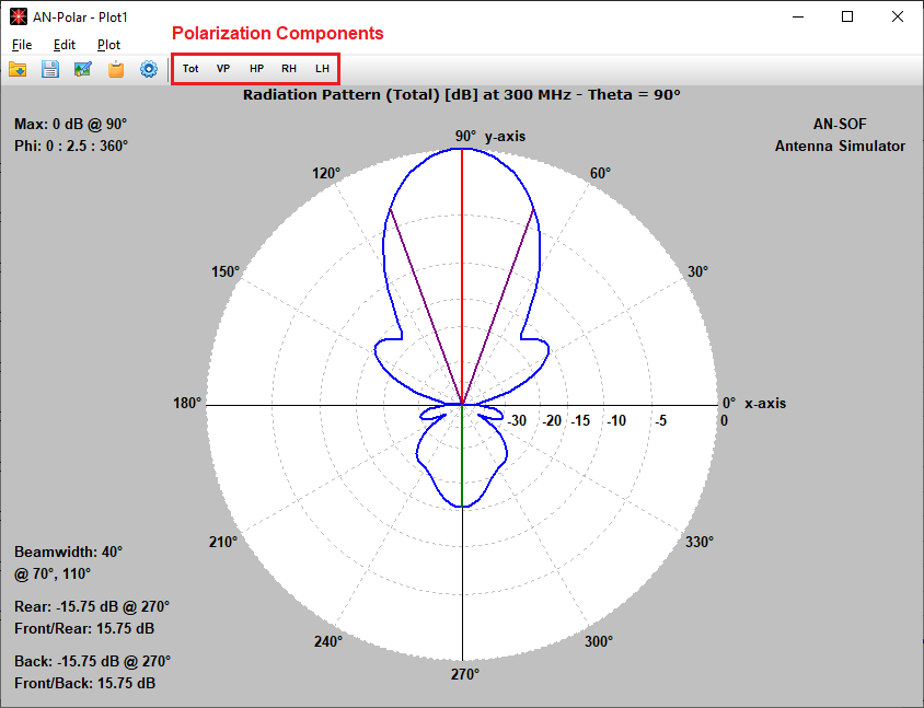
For a classic representation of antenna performance, the far-field pattern can be visualized in a 2D polar chart by selecting Results > Plot Far-Field Pattern > Polar Plot 1 Slice from the AN-SOF main menu (Fig. 3). This action launches the AN-Polar application, a dedicated environment for analyzing directional characteristics.
Polarization and Multi-Slice Analysis
The AN-Polar interface includes a specialized toolbar with buttons (Tot, VP, HP, RH, LH) that allow for the immediate decomposition of the pattern into its respective linear or circular polarization components.
To compare different planes of radiation simultaneously:
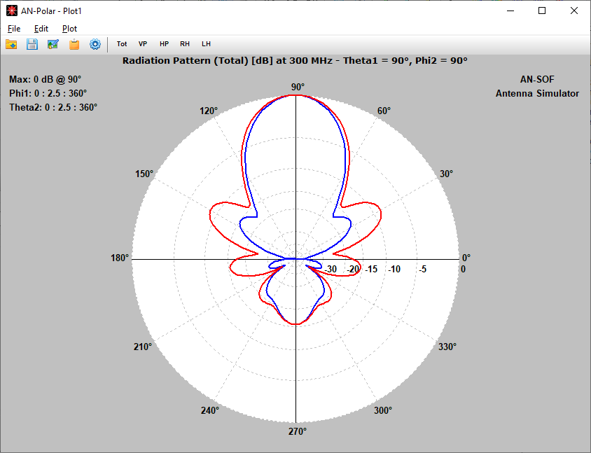
- Navigate to Results > Plot Far-Field Pattern > Polar Plot 2 Slices.
- Use the resulting dialog box (Fig. 4) to overlay two distinct slices on a single chart.
- Available combinations include two vertical slices (E and H planes), two conical slices, or a vertical-conical hybrid view.
Interactive Metrics and Auto-Calculation
AN-Polar provides real-time data feedback. Clicking any point on the polar curve displays the specific metric value and its associated polar angle. When a single slice is plotted, the software automatically calculates and displays key performance metrics in the lower-left corner:
- Beamwidth: The angular width between the -3 dB points.
- Front-to-Back (F/B) Ratio: The ratio of power in the primary lobe to that at exactly 180°.
- Front-to-Rear (F/R) Ratio: The ratio of the main lobe to the maximum level in the entire rear hemisphere (worst-case scenario).
See Also:
Customization and Scaling (AN-Polar Preferences)
The Preferences window (Fig. 5), accessible via the Edit menu or the gear icon, allows for deep customization of the visual output, including title editing, line thickness, font selection, and plot rotation.
A critical feature within this window is the Scale Type selection:
- Linear (Lin): A standard “textbook” scale where radial distances are divided into equal intervals.
- Logarithmic (Log): An “ARRL-style” log scale. This scale follows the traditional standards used in ARRL publications and handbooks. It is particularly advantageous for antenna designers as it expands the visualization of small secondary lobes and nulls that are often compressed and difficult to resolve in a linear scale.
