Search for answers or browse our Knowledge Base.
Guides | Models | Validation | Book
AN-SOF Overview
Features and Capabilities
AN-SOF is a comprehensive software tool for the modeling and simulation of antenna systems and radiating structures in general.
AN-SOF is intended for solving problems in the following areas:
- Modeling and design of wire antennas.
- Antennas above a lossy ground plane.
- Broadcast antennas over radial wire ground screens.
- Single layer microstrip patch antennas.
- Radiated emissions from printed circuit boards (PCBs).
- Electromagnetic Compatibility (EMC) applications.
- Passive circuits, transmission lines, and non-radiating networks.
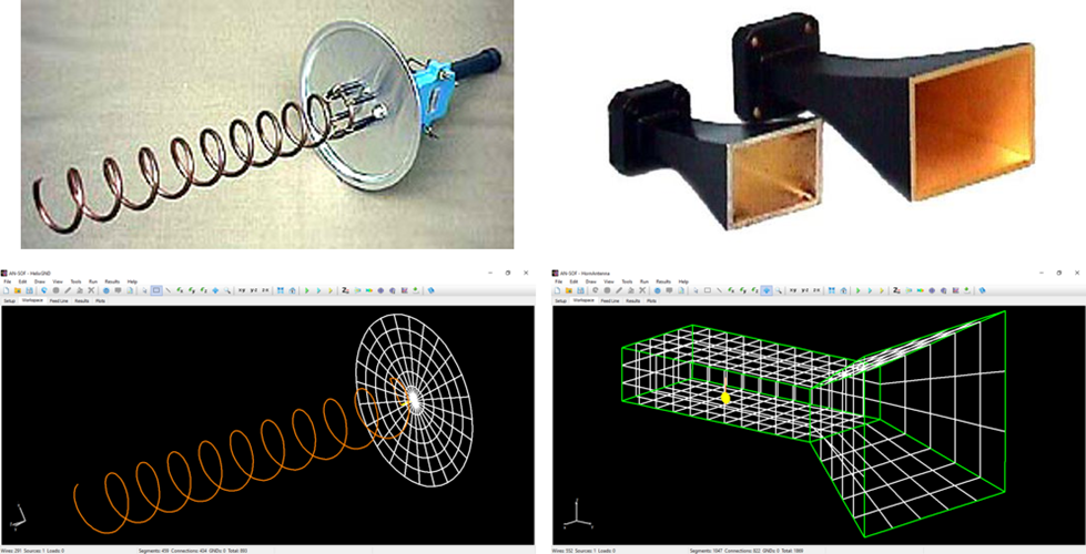
AN-SOF is based on an improved version of the so-called Method of Moments (MoM) for wire structures. Metallic objects like antennas can be modeled by a set of conductive wires and wire grids, as it is illustrated in Fig. 1. In the MoM formulation, the wires composing the structure are divided into segments that must be short compared to the wavelength. If a source is placed at a given location on the structure, an electric current will be forced to flow on the segments. The induced current on each individual segment is the first quantity calculated by AN-SOF.
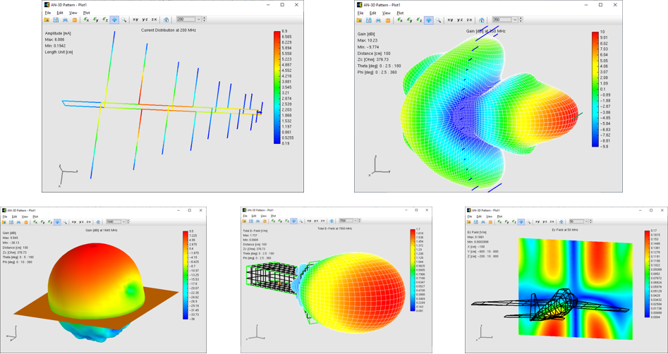
Once the current distribution has been obtained, the radiated electromagnetic field can be computed in the far- and near-field zones. Input parameters at the position of the source or generator can also be obtained, such as the input impedance, input power, standing wave ratio (SWR), reflection coefficient, transmission loss, etc.
The modeling of the structure can be performed by means of the AN-SOF specific 3D CAD interface. Electromagnetic fields, currents, voltages, input impedances, consumed and radiated powers, directivity, gain and many more parameters can be computed in a frequency sweep and plotted in 2D and 3D graphical representations.
In the case of curved antennas like loops, helices, and spirals, the MoM in AN-SOF has been improved to accurately account for the wire’s exact curvature. Traditional calculations often use straight-line segments to approximate curved antennas, resulting in many discontinuous wire junctions. This linear approximation can be inefficient in terms of computer memory and the number of calculations required, as it necessitates multiple straight segments to mimic the smooth curvature of wires. To address this issue, AN-SOF uses curved segments that precisely follow the contours of curved antennas. This innovative technique is known as the Conformal Method of Moments (CMoM).
As an example, Fig. 2 shows the different approaches to a circular disc obtained by means of the MoM and CMoM methods. Both methods are available in AN-SOF since the MoM is a special case of the more general CMoM.
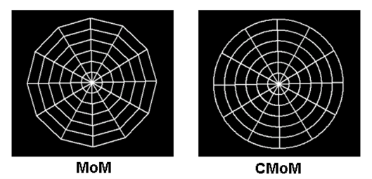
In addition to the CMoM capabilities, advanced mathematical techniques have been implemented in the calculation engine making possible simulations from extremely low frequencies (e.g., electric circuits at 50-60 Hz) to very high ones (e.g., microwave antennas above 1 GHz).
In what follows, a summary of the modeling options and the simulation results that can be obtained from AN-SOF is presented.
Modeling of Metallic Structures
Metallic structures can be modeled by combining different types of wires, grids, and surfaces:
Wires
Wire Grids and Solid Surfaces
- All types of curved wires can be modeled by means of arced or quadratic segments.
- Wire grids and solid surfaces can be defined using either curved or straight wire segments. Curved segments follow the exact curvature of discs, rings, cones, cylinders, spheres, and parabolic surfaces. Grids are composed of cylindrical wires that leave holes between them, while solid surfaces are composed of flat wires or strips that cover the surface without leaving holes between them.
- Tapered wires with stepped radii can be defined.
- All wires can be loaded or excited at any segment.
- The structure can also have finite non-zero resistivities (skin effect).
- Electrical connections of different wires and connections of several wires at one point are possible.
- Metallic wires in either dielectric or magnetic media can be analyzed.
- Wires with insulation can be modeled. Dielectric and magnetic coatings are available.
- The structures can be placed in free space, over a perfectly conducting ground plane or over an imperfect ground plane.
- Flat strip lines can be defined on a dielectric substrate for modeling planar antennas and printed circuit boards (PCB).
- Vias in microstrip antennas and printed circuit boards can also be modeled.
- The wire cross-section can either be Circular, Square, Flat, Elliptical, Rectangular or Triangular.
- Transmission lines can be connected to the metal structure. There are over 160 cable models available, including two-wire and coaxial cables, with characteristic impedance, velocity factor, and loss parameters adjusted to actual datasheets.
- The geometry modeling can be performed in suitable unit systems (um, cm, mm, m, in, ft). Different unit systems can also be chosen for inductance (pH, nH, uH, mH, H) and capacitance (pF, nF, uF, mF, F).
Excitation Methods
- Voltage sources can be placed on the wires, as many as there are segments, with equal or different amplitudes (RMS values) and phases.
- Current sources (e.g., representing impressed currents) can also be arranged at any segments.
- The voltage and current sources can have internal impedances.
- An incident plane wave of arbitrary polarization (linear, circular, or elliptical) and direction of incidence can also be used as the excitation.
- Hertzian electric and magnetic dipoles can also be modeled and used as the excitation.
- The antenna input power can be set to obtain the results (current distribution, near and far fields) scaled accordingly.
Frequency options
- The simulation can either be performed for a single frequency, for frequencies taken from a list or for a frequency sweep.
- The list of frequencies can either be created inside the program or loaded from a text file. It can also be saved to a txt file.
- Linear and logarithmic frequency sweeps are possible.
- A suitable unit system can be selected (Hz, KHz, MHz, GHz).
Data Input
- 3D CAD tools are implemented for drawing and modifying the structure geometry, including wires, grids, surfaces, discrete generators, and lumped loads.
- The segmentation of wire geometry can be done automatically or manually.
- Left-clicking on a wire selects and highlights it. Right-clicking on a wire reveals a pop-up menu with various options.
- Wire connections are easily established by copying and pasting the endpoints of wires.
- Special 3D symbols indicate the positions of sources, load elements, and ground points.
- All dialog boxes validate inputs for accuracy.
- The program includes mouse-supported functions for rotating, moving, and zooming.
- Transmission lines can be easily entered into a table, which serves as a library, for later use. A line is highlighted in the graphical interface for easy identification.
- The program allows you to import geometrical data from text files. It supports three different file formats for importing wires, including the NEC (Numerical Electromagnetics Code) cards. Additionally, it can import DXF files containing 3D LINE entities.
- The AN-SOF architecture integrates powerful numerical methods to achieve the fastest calculation speed and the most accurate results.
Data Output
- All computed data is stored in files for subsequent graphical analysis.
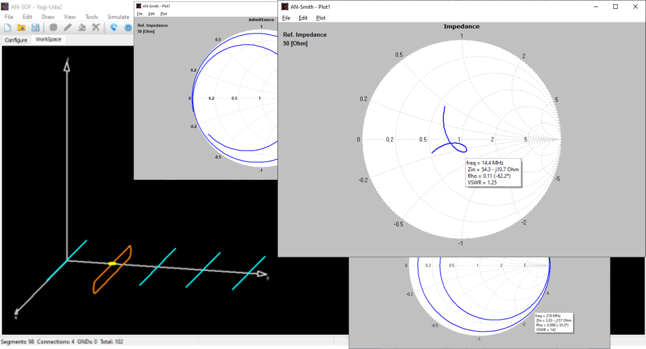
- Input impedances, currents, voltages, VSWR, S11, return and transmission losses, radiated and consumed powers, efficiency, directivity, gain, and other system responses are presented as lists in text format and can be plotted against frequency. A Smith chart is available to represent impedances and admittances, as well as to display the reflection coefficient and VSWR at the selected point on the graph.
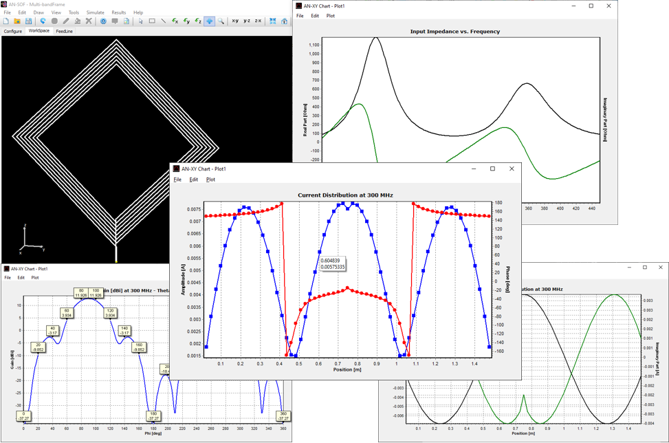
- The current distribution on a selected wire can be plotted in amplitude, phase, real, and imaginary parts against position in a 2D representation. The currents flowing on a structure can also be plotted as a color map on the wires.
- Radiation and scattering fields are obtained, including power density, directivity and gain patterns, total electric field, linearly and circularly polarized components, axial ratio, and Radar Cross Section (RCS). The surface-wave field can be determined as a function of distance in the case of a real ground with finite conductivity.
- Near-field components can be calculated in Cartesian, cylindrical, and spherical coordinates. Field intensities can be plotted in 2D and 3D graphical representations and visualized as color maps in the proximity of a structure.
- A 2D representation of radiated fields is available in Cartesian and polar coordinates. The ARRL-style log scale can be applied to polar diagrams.
- 3D radiation patterns can be viewed from arbitrary angles with zoom functions, colored mesh and surface representations, and a color bar scale. 3D patterns can be plotted with specially designed lighting and illumination for enhanced visualization of simulation results.
- Far-field patterns can be separated into theta (vertical) and phi (horizontal) linearly polarized components, as well as right and left circularly polarized components. The axial ratio and the front-to-rear and front-to-back ratios are shown in polar plots and can be displayed as a function of frequency.
- The frequency spectrum of near- and far-fields can be visualized in a 2D representation for all field components across different frequencies.
- An average radiated power test, also known as AGT (Average Gain Test), is conducted to verify the accuracy of the simulation.
- The calculated data can be exported to .csv, .dat, or .txt files for use in other software programs.
- An embedded transmission line calculator is included to simplify the design of feed lines for transmitting antennas. Actual cable part numbers can be selected from a wide range of manufacturers, thanks to data extracted from cable datasheets and integrated into the calculator.
- A Bulk Simulation feature enables the automated calculation of multiple files, each with different geometric descriptions, to obtain results based on variable geometric parameters. The results are automatically exported to .csv files for further processing.
- You can choose suitable unit systems for the plotted results, including current scaling (KA, A, mA, uA), voltage scaling (KV, V, mV, uV), electric field scaling (KV/m, V/m, mV/m, uV/m), magnetic field scaling (KA/m, A/m, mA/m, uA/m), decibel scales, and more.
Integrated graphical tools
AN-SOF has a suite of integrated graphical tools for the convenient visualization of the simulation results. The following applications are installed automatically and used by the main program, AN-SOF:
AN-XY Chart app
A friendly 2D chart for plotting two related quantities, Y versus X. Use AN-XY Chart to plot parameters that depend on frequency, such as currents, voltages, impedances, reflection coefficient, VSWR, S11, radiated power, consumed power, directivity, gain, radiation efficiency, radar cross section, field components, axial ratio, and many more. Also plot the current distribution along wires as a function of position, 2D slices of radiation lobes and near fields as a function of distance from an antenna. Choose different units to display results and use the mouse to easily zoom and scroll graphs.

AN-Smith app
Plot impedance or admittance curves on the Smith chart with this tool. Just click on the graph to get the frequency, impedance, reflection coefficient, VSWR, and S11 that correspond to each point on the curve. Plots can be stored in independent files and opened later for a graphical analysis with AN-Smith.

AN-Polar app
Plot on a polar diagram the radiation pattern versus the azimuth (horizontal) or zenith (vertical) angles. The maximum, -3dB and minimum radiation levels are shown within the chart as well as the beamwidth and front-to-rear/back ratio. Click on the graph to quickly obtain the values of the radiated field. The represented quantities include power density, directivity, gain, normalized radiation pattern, total electric field, linearly and circularly polarized components, axial ratio, and radar cross section (RCS).
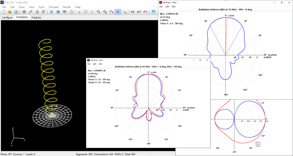
AN-3D Pattern app
Get a complete view of the radiation properties of a structure by plotting a 3D radiation pattern. AN-3D Pattern implements colored mesh and surface for the clear visualization of radiation lobes, including a color bar-scale indicating the field intensities over the lobes. Quickly rotate, move, and zoom the graph using the mouse. The 3D radiation pattern can be superimposed to the structure geometry to gain more insight into the directional properties of antennas.
The represented quantities include the power density, normalized radiation pattern, directivity, gain, total field, linearly and circularly polarized components, axial ratio, and Radar Cross Section (RCS). Choose between linear or decibel scales. Display near fields as color maps in the proximity of antennas in three different representations: Cartesian, cylindrical and spherical plots. Also plot the current distribution on the structure as a colored intensity map.