Helical Antennas in Normal Mode: Theoretical Limits and Numerical Validation

Created OnOctober 31, 2022

Updated OnFebruary 4, 2026

By:Tony Golden

Validate the electromagnetic behavior of the helical antenna in its Normal Mode through this detailed study referencing the foundational work of John D. Kraus. By analyzing the transition from a 3D helical structure to its theoretical loop-dipole equivalent, this article demonstrates how AN-SOF accurately captures the broadside radiation pattern and the asymptotic gain limit. Essential reading for engineers and designers modeling compact curved radiators and electrically small antennas.

Introduction and Geometric Definitions

The helical antenna is a fundamental electromagnetic structure consisting of a conducting wire wound in the form of a screw thread. To analyze its performance, we must first establish its geometric parameters relative to the operating wavelength ($\lambda$).

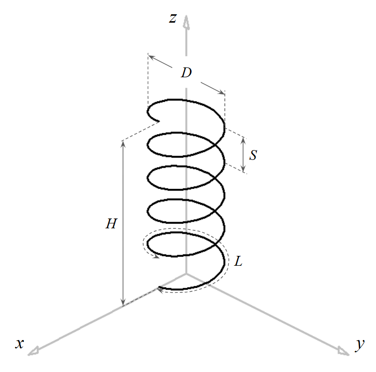
The helix geometry is defined by the following variables (Fig. 1):

Radius ($R$): The distance from the axis to the center of the wire. The helix diameter is $D = 2R$.
Circumference ($C$): The length of a single turn in the plane perpendicular to the axis, where $C = 2\pi R$.
Spacing ($S$): The axial distance between adjacent turns, also known as the pitch.
Number of turns ($N$): The total count of full revolutions in the helix.
Pitch Angle ($\alpha$): The angle between a line tangent to the helix wire and the plane perpendicular to the helix axis.

**Fig. 1:** A right-handed helix indicating key geometric parameters.

The pitch angle can be calculated as:

$\displaystyle \alpha \,=\, \arctan\left(\frac{S}{C}\right)$

Modes of Operation

As established by Prof. John D. Kraus in his definitive work, Antennas (2nd Edition, McGraw-Hill, 1988), the helical antenna operates in two primary modes depending on its electrical size:

Normal Mode (Broadside Mode): This occurs when the helix is electrically small, specifically when the circumference $C \ll \lambda$ and the spacing $S \ll \lambda$. In this mode, the maximum radiation occurs in the plane normal to the helix axis.
Axial Mode (End-fire Mode): This occurs when the circumference $C$ is approximately one wavelength ($C \approx \lambda$). In this mode, the maximum radiation occurs along the axis of the helix.

This article focuses on the validation of the Normal Mode. Under these electrically small conditions, the current distribution along the wire can be considered uniform, allowing the helix to be modeled as a combination of a small loop (representing the transverse component) and a short dipole (representing the axial component).

Principles of the Normal Mode

In the Normal Mode, the helix acts as a composite radiator. The far-field is the superposition of the fields produced by the equivalent loops and dipoles. The radiation pattern is broadside, meaning it is at its maximum in the $xy$-plane if the helix axis is aligned with the $z$-axis.

If the dimensions are specifically chosen such that $C = \sqrt{2S\lambda}$, the radiation becomes circularly polarized. However, for the purpose of theoretical validation, we look at the limiting case where the helix dimensions shrink toward zero. As the pitch ($S$) and circumference ($C$) decrease, the antenna converges toward the behavior of an infinitesimal “combined” radiator.

Numerical Simulation and Results

The validation was performed using the Conformal Method of Moments (CMoM) in AN-SOF at a frequency of 299.8 MHz. This makes dimensions in meters equivalent to dimensions measured in wavelengths, since $\lambda \approx 1 \text{ m}$.

A perfectly electrically conducting (PEC) ground plane is situated in the $xy$-plane, and the helix is positioned above it, with its axis aligned along the $z$ axis. This setup allows for excitation by connecting a source to a short vertical wire running from the helix base to the ground plane, which acts as a counterpoise. Consequently, radiation is confined to the upper half-space.

Radiation Pattern Analysis

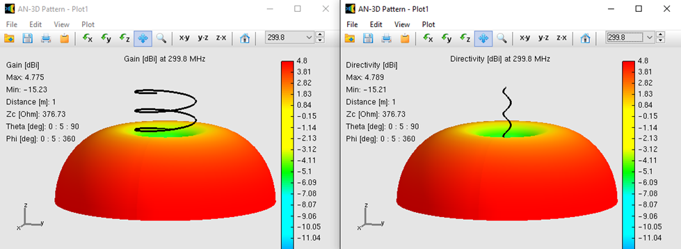
The computed broadside radiation pattern, shown in Fig. 2, illustrates the gain in dBi of a small helix above a PEC ground plane. The helix has a circumference $C/\lambda = 0.01$, $N = 5$ turns, and two pitches: $S = 0.001\lambda$ (left) and $S = 0.01\lambda$ (right).

As predicted by theory, the maximum gain is located in the plane perpendicular to the axis, and the radiation pattern is “donut-shaped,” with nulls along the $z$-axis. The numerical stability of the CMoM engine ensures that the curved contour of the helix is modeled exactly, rather than using a series of linear staircase approximations.

**Fig. 2:** Gain pattern (in dBi) of a small helical antenna situated above a perfect ground plane. The plots compare two configurations: 5 turns with a pitch of $0.001\lambda$ (left) and 5 turns with a pitch of $0.01\lambda$ (right), both for a circumference-to-wavelength ratio ($C/\lambda$) of 0.01.

The Asymptotic Gain Limit

A key aspect of this validation is the determination of peak gain as the helix becomes infinitesimal. For a small helix with uniform current, the directivity is equivalent to that of a combined small loop and short dipole.

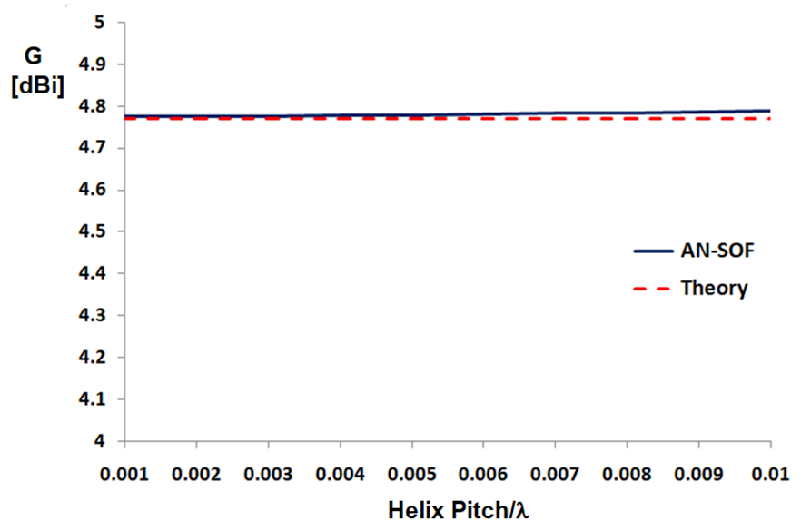
Figure 3 shows the peak gain plotted as a function of the pitch ($S$) measured in wavelengths. As the pitch tends toward zero, the calculated gain converges to $4.77 \text{ dBi}$.

This value confirms the theoretical prediction. A gain of $4.77 \text{ dBi}$ is equivalent to a factor of $3$ ($10 \log_{10}(3) \approx 4.77$). Since a standard infinitesimal dipole or small loop has a gain of $1.76 \text{ dBi}$ (a factor of $1.5$), placing it just above a PEC ground plane results in exactly twice the power density, for a total gain factor of $2 \times 1.5 = 3$.

**Fig. 3:** Gain of a small helix antenna with 5 turns ($N = 5$) above a perfect ground plane as a function of the pitch in wavelengths ($S/\lambda$). The circumference is $C/\lambda = 0.01$.

Conclusions

The analysis of the helical antenna in Normal Mode provides a rigorous validation of the AN-SOF simulation engine against the classical experimental and theoretical data provided by John D. Kraus. Several critical conclusions can be drawn:

Geometric Precision: The simulation successfully models the transition from a complex 3D helical wire to its functional equivalent of a loop-dipole pair. The use of CMoM allows for the exact representation of the helix curvature, which is essential for capturing the precise phase relationships between the loop and dipole components.
Theoretical Correlation: The convergence of the gain to 4.77 dBi as the pitch ($S/\lambda$) approaches zero (Fig. 3) provides an exact numerical match to the theoretical limiting case of an infinitely small helix. This proves that the solver correctly calculates electromagnetic interactions for electrically small curved elements.
Broadside Stability: The radiation patterns (Fig. 2) confirm that the Normal Mode’s broadside characteristic is accurately maintained for small circumferences. The absence of numerical artifacts in the nulls along the helix axis demonstrates the high dynamic range and precision of the software’s exact kernel.

Ultimately, these results confirm that AN-SOF is a robust tool for modeling compact helical radiators. For applications such as low-frequency sensing where gain optimization is critical, the software successfully bridges the gap between the foundational experiments of the 20th century and the rigorous requirements of modern, high-precision antenna engineering.