Search for answers or browse our Knowledge Base.
Guides | Models | Validation | Book
Validating Dipole Antenna Simulations: A Comparative Study with King-Middleton
This article presents a comprehensive comparison between AN-SOF’s dipole antenna simulations and the renowned King-Middleton second-order solution. Through rigorous analysis and numerical experiments, we validate the accuracy and reliability of AN-SOF in predicting dipole antenna input impedance.
Introduction
Cylindrical antennas have been the subject of extensive theoretical and experimental research for decades. As a result, a wealth of data exists on the input impedance of linear antennas. In this article, we will compare the simulation results obtained using AN-SOF Antenna Simulation Software with these established theoretical values. This comparison serves as a crucial validation step, not only for dipole antennas but also for dipole antenna arrays like Yagi-Uda antennas and Log-Periodic Dipole Arrays (LPDA).
The King-Middleton Second-Order Solution
For our theoretical comparison, we have selected the King-Middleton solution as presented in Ronold W. P. King’s seminal work, “The Theory of Linear Antennas” (Harvard University Press, 1956). This second-order solution, based on an iterative approach to the solution of an integral equation involving sinusoidal functions for the current distribution, remains a highly regarded analytical benchmark in the field of antenna design.
While the King-Middleton solution offers a sophisticated approach, it does introduce certain simplifications. The delta-gap source model, which assumes an infinitesimal gap at the feed point and an infinitely strong electric field, neglects edge effects in the terminal zone. Despite this limitation, the second-order solution has demonstrated remarkable accuracy in predicting input impedance values when compared to experimental data.
Given its theoretical rigor and historical significance, the King-Middleton second-order solution serves as an ideal reference for validating numerical methods. In the following section, we will present simulation results for cylindrical antennas of varying lengths and thicknesses, comparing the input impedance calculated by AN-SOF to the King-Middleton values.
Comparing AN-SOF Results with King-Middleton
Figure 1 depicts the geometry of a center-fed cylindrical antenna with length $L = 2h$ and radius $a$, aligned with the $z$-axis. The diagram highlights the field components $E_z$ and $H_\phi$, which are essential for calculating input impedance. Additionally, it identifies the electric current element $I(z’) dz’$ employed in integral equation formulations to solve for the dipole impedance.
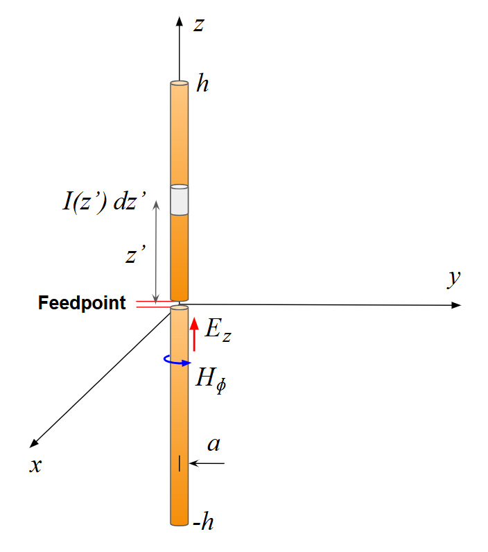
Figure 2 displays the input impedance of the dipole antenna plotted against its normalized half-length, $\beta h$ (expressed in radians). In this context, $\beta = 2\pi/\lambda$ represents the wavenumber, $h$ is the physical half-length of the dipole, and $\lambda$ denotes the free-space wavelength.
The antenna thickness varies across three cases for the conductor radius: (a) $a/\lambda$ = 0.001191, (b) $a/\lambda$ = 0.003175, and (c) $a/\lambda$ = 0.009525. For a wavelength $\lambda$ = 1 m (39.37 inches), these correspond to a diameter of (a) 3/32″, (b) 1/4″, and (c) 3/4″. The blue solid lines represent AN-SOF simulation results, while the red dashed lines depict King-Middleton second-order solution (refer to Table 30.12 of King’s book).
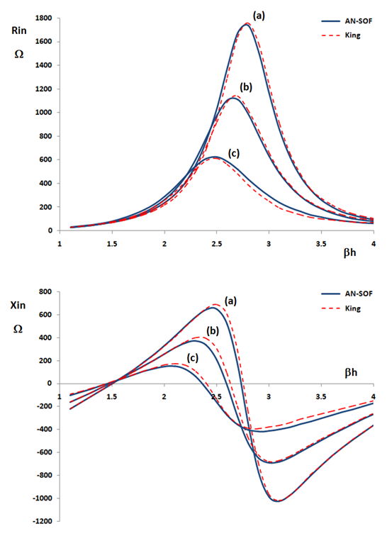
To account for the finite gap effect neglected by King’s model, three different gap sizes were introduced in the AN-SOF simulations: (a) 0.02$\lambda$, (b) 0.04$\lambda$, and (c) 0.1$\lambda$. This was achieved by inserting a short wire segment of the corresponding length at the feed point where the source was connected.
The excellent agreement between the AN-SOF simulations and King’s results, particularly for smaller gap sizes, validates the accuracy of AN-SOF’s dipole antenna modeling and confirms the robustness of the King-Middleton solution, even with its inherent limitations.
Model Refinement and Convergence Analysis
Figure 3 illustrates the AN-SOF model on the left. To maintain a consistent segment length of 0.02$\lambda$ throughout the simulation, the number of segments was increased as $\beta h$ grew. This segment length proved to be sufficient for achieving convergence in the input impedance calculations.
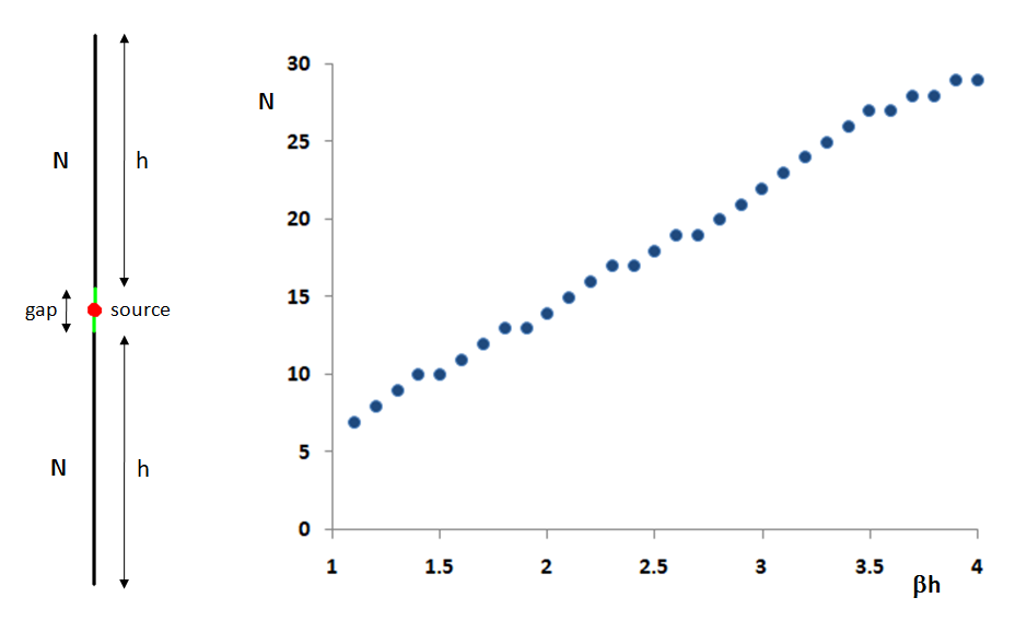
The right side of Fig. 3 depicts the number of segments, N, used in each arm of the cylindrical antenna as a function of $\beta h$. The linear relationship is a direct result of our deliberate choice to maintain a constant segment length of 0.02$\lambda$. This corresponds to 50 segments per wavelength.
As evidenced in Fig. 2, the excellent agreement between the King-Middleton second-order approximation and AN-SOF’s results further validates the accuracy of our modeling approach and the robustness of both theoretical and numerical methods for dipole antenna analysis.
Concluding Remarks and Additional Data
As a supplement to this article, we present results from Ronald J. Stockton (callsign N0RR), a user who has independently implemented the King-Middleton second-order solution. Ron’s findings corroborate our earlier conclusions. Using a total of 45 segments (22 on each arm and 1 at the center) in AN-SOF, the input impedance converges to the King-Middleton second-order solution implemented by Ron in his own code, demonstrating the accuracy achieved by AN-SOF.
The table below summarizes the results as a function of $\Omega$, Hallen’s expansion parameter, which quantifies the antenna’s thickness, and it is given by
$\displaystyle \Omega \,=\, 2\,\ln\left( \frac{2h}{a}\right)$
Click the button below the table to download an Excel file containing the complete data, including values from King’s book, Ron’s code, and AN-SOF for 45 segments.
| $\beta h$ | $\Omega$ | K-M 2nd order | AN-SOF (45 seg) | ||
| — | — | R | X | R | X |
| 1.2 | 10* | 37.842 | -127.001 | 36.502 | -128.026 |
| 1.4 | 10* | 59.153 | -34.307 | 59.606 | -35.916 |
| 1.6 | 10* | 91.403 | 54.582 | 97.586 | 54.03 |
| 1.2 | 12.5 | 37.134 | -185.797 | 36.396 | -185.516 |
| 1.4 | 12.5 | 57.384 | -60.07 | 57.477 | -60.292 |
| 1.6 | 12.5 | 87.655 | 60.400 | 90.366 | 61.064 |
| 1.2 | 15 | 36.742 | -244.013 | 36.27 | -244.44 |
| 1.4 | 15 | 56.36 | -86.012 | 56.25 | -86.706 |
| 1.6 | 15 | 85.404 | 65.397 | 86.472 | 65.119 |
| 1.2 | 20 | 36.336 | -361.567 | 36.112 | -330.1 |
| 1.4 | 20 | 55.248 | -138.041 | 55.066 | -139.258 |
| 1.6 | 20 | 82.88 | 74.476 | 83.039 | 73.264 |
It’s always gratifying to receive feedback from customers who share their insights on the accuracy of AN-SOF. Below is Ron’s comparison, highlighting how AN-SOF performs against the King-Middleton (K-M) theoretical standard and NEC engines:
Hello Tony,
You may be interested in my analysis tool comparisons for the impedance of two dipole lengths: halfwave and near resonance with a practical value of Ω = 12.5.
The King-Middleton 2nd-order solution is probably still the ‘gold standard’ for theoretical results.
- AN-SOF converges to the K-M solution for X around 39 & 45 segments.
- NEC4.2 does not converge to the K-M solution by changing the number of segments.
- NEC5-x13 converges for the K-M X value around 42 segments.
- Both NEC versions have the wavelength offset from conventional wisdom.
BTW – I now use AN-SOF for all my Yagi analyses and designs.
Ron Stockton (N0RR)
Keep up the good work,
Ron Stockton’s Biography
Ronald J. Stockton (N0RR) has over 40 years of experience as an antenna engineer and department manager at Hughes Aircraft and Ball Telecommunications Products, specializing in advanced active aperture phased arrays. He holds multiple patents for monolithic microstrip phased arrays on GaAs substrates operating at 20 GHz receive and 44 GHz transmit frequencies. Having previously used NEC software, Ron has transitioned to AN-SOF to design 6-, 7-, and 8-element OWA Yagis with a 50 Ohm input impedance across a 2.8% bandwidth for the amateur radio community.
See Also:
Technical Keywords: Dipole Antenna, King-Middleton Second-Order Solution, Input Impedance, Method of Moments (MoM), Numerical Validation, Cylindrical Antenna, Hallen’s Expansion Parameter, Computational Electromagnetics, Antenna Modeling, Simulation Convergence, RF Engineering.
