Quick Start Guide

Enhancing Antenna Design Through Simulation Software

An antenna model represents a real-world antenna within a computer program. It is important not to confuse this type of model with a scale model, which is sometimes constructed to measure the radiation characteristics of a larger, physically identical antenna. Due to the mathematical complexity involved in modeling, specialized software is often used to predict and analyze antenna performance.

Computer simulation plays a critical role in overcoming challenges and driving innovation throughout the product development lifecycle. A computer model offers significant advantages, including the ability to modify, redesign, break, destroy, and rebuild designs multiple times without wasting physical materials. By leveraging simulation software, engineers can significantly reduce the costs associated with building successive physical prototypes, streamlining the design process.

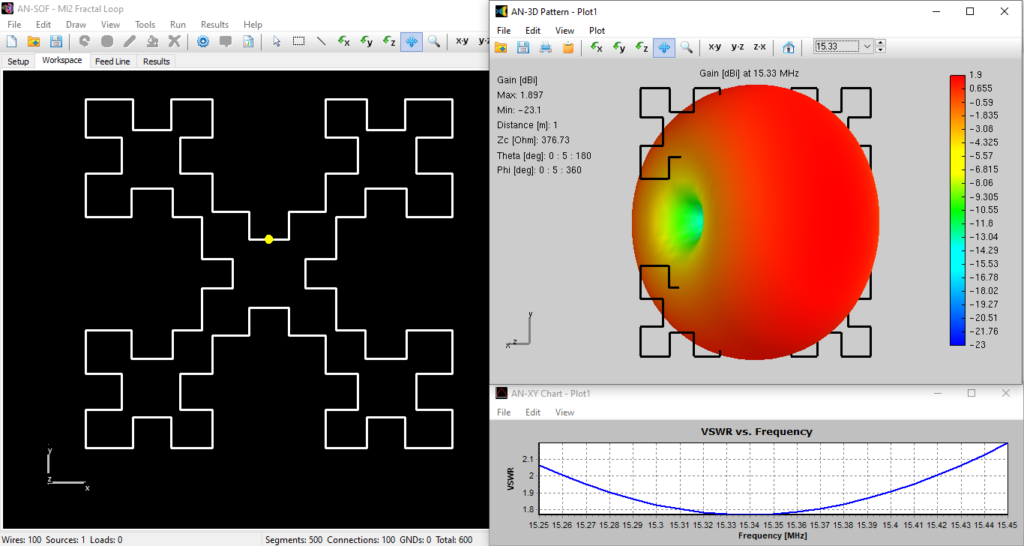
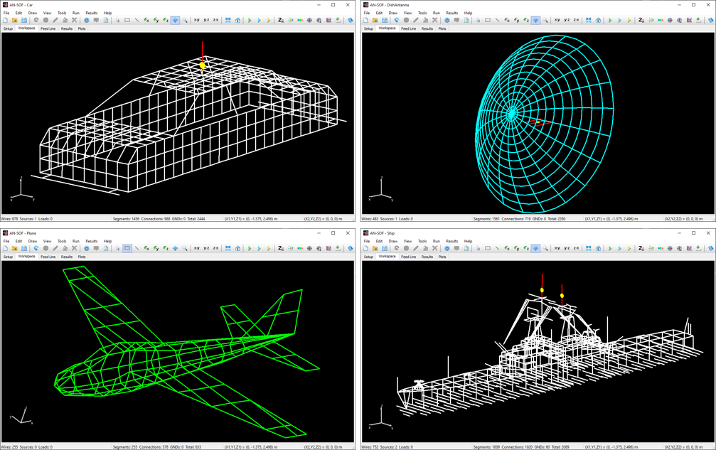
AN-SOF is a comprehensive simulation software suite designed for antenna modeling and optimization. It supports the design of a wide range of wire antennas, including dipoles, monopoles, Yagis, log-periodic arrays, helices, spirals, loops, horns, fractals, phased arrays, and many other types. Additionally, AN-SOF enables detailed modeling of feeding systems using transmission lines, allowing users to analyze complex antenna configurations with precision. The software can simulate antennas positioned above lossy ground planes or broadcast antennas above radial wire ground screens, providing realistic and accurate results.

Furthermore, AN-SOF’s calculation capabilities have been extended to include single-layer microstrip patch antennas and the computation of radiated emissions from Printed Circuit Boards (PCBs). As a result, AN-SOF is a powerful tool for Electromagnetic Compatibility (EMC) applications. The software also supports passive circuits with lumped impedances and non-radiating networks, enabling comprehensive analysis of antenna systems.

Note

In the realm of antenna applications, AN-SOF proves invaluable as it empowers users to achieve the following:

• Design superior antennas.
• Predict and optimize antenna performance.
• Fine-tune antenna parameters for optimal results.
• Account for environmental effects on antenna performance.
• Employ script-based optimization to refine designs.
• Gain valuable insights into antenna behavior.
• Experiment multiple times prior to physically building the antenna model.
• Deepen understanding of antennas and their properties.
• Facilitate knowledge sharing and collaboration with colleagues.

With AN-SOF at your disposal, you can explore the exciting possibilities of antenna analysis and optimization. The software provides an extensive toolkit for designing, evaluating, and enhancing antenna performance, empowering engineers and enthusiasts alike to push the boundaries of innovation.

Note

AN-SOF enables us to perform a wide range of tasks, including:

• Describing the antenna’s geometry accurately.
• Selecting appropriate construction materials.
• Specifying the environmental and ground conditions.
• Determining the antenna’s height above the ground.
• Analyzing the radiation pattern and front-to-back ratio.
• Plotting directivity and gain.
• Evaluating impedance and SWR (Standing Wave Ratio).
• Predicting bandwidth.
• Obtaining numerous additional parameters and plots.

Drawing the geometry of structures in AN-SOF is intuitive and user-friendly. Wires can be created in a 3D space using the mouse, menus, and easy-to-navigate dialog windows. Tools are available to zoom, move, and rotate the structure, ensuring precise control over the design process.

To visualize simulation results, AN-SOF integrates seamlessly with a suite of specialized applications: AN-XY Chart, AN-Smith, AN-Polar, and AN-3D Pattern. These tools allow users to display graphs and analyze data effectively. They can also be executed independently for further graphic processing, offering flexibility and convenience for advanced users.

Introduction to AN-SOF: Antenna Simulation Essentials

AN-SOF performs computations of electric currents flowing on metallic structures, including antennas in transmitting and receiving modes, as well as scatterers. A scatterer refers to any object capable of reflecting and/or diffracting radiofrequency waves. For instance, wave scattering analysis can be conducted on the surface of an aircraft to determine optimal antenna placement, on a parabolic reflector to examine gain in relation to the reflector shape, or on a car’s chassis to predict interference effects.

The Method of Moments (MoM) stands as one of the most widely validated techniques for antenna simulation. AN-SOF incorporates an enhanced and advanced version of this method called the Conformal Method of Moments (CMoM) with Exact Kernel, which addresses various challenges associated with traditional MoM approaches and achieves unparalleled accuracy.

Interested in learning more about the CMoM implementation in AN-SOF? Read this article:

• Overcoming 7 Limitations in Antenna Design: Introducing AN-SOF’s Conformal Method of Moments

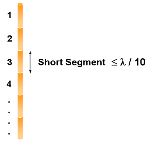
According to the MoM, any metallic structure can be represented using conductive wires, as illustrated in Fig. 1. These wires are subdivided into small segments, which assume the shape of cylindrical tubes. To obtain accurate results, the length of each wire segment should be comparatively short compared to the wavelength, as depicted in Fig. 2. However, this concern can be alleviated during the initial simulation since AN-SOF automatically handles the segmentation of wires.

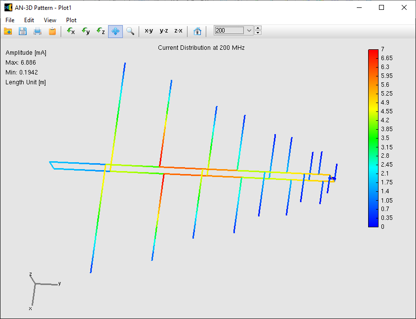
The flow of electric currents within the structure can be achieved by introducing a voltage generator at a specific location operating at a given frequency. Current generators can also serve as the excitation source, alongside plane waves impinging on the structure from distant sources. Once the geometry, materials, and sources of the structure are defined, the computation can be executed to determine the currents flowing through the wire segments. Generally, these electric currents exhibit varying intensities along and across the structure, collectively referred to as a current distribution. Fig. 3 showcases an example of the current distribution on a log-periodic antenna.

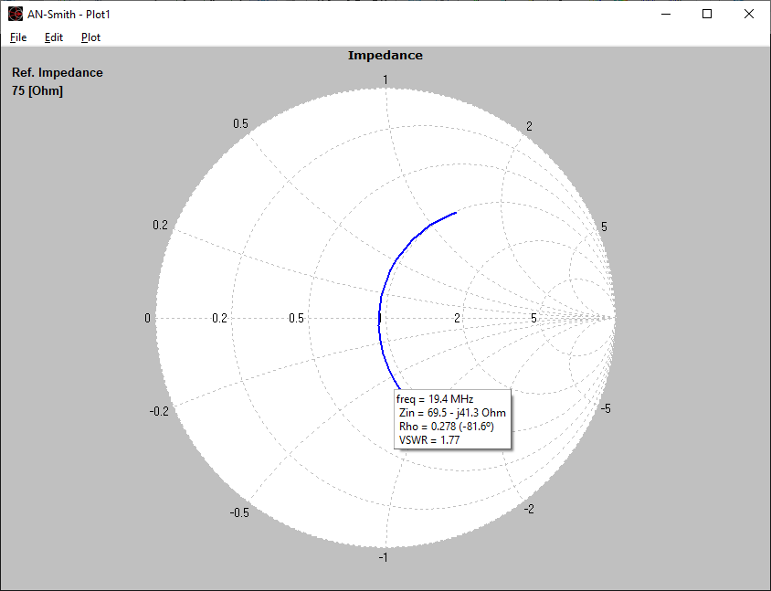
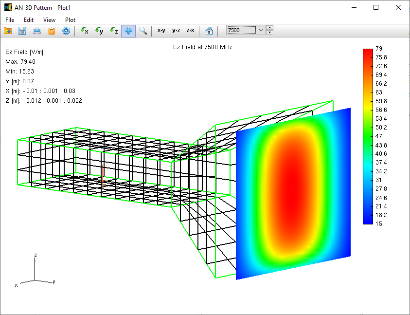
In the subsequent phase of the simulation process, the electromagnetic field radiated by the current distribution can be calculated. However, the current distribution itself provides valuable insights into the behavior of the structure, particularly when a frequency sweep is conducted. In the case of antennas, the feed point impedance can be analyzed as a function of frequency to assess the bandwidth. The Voltage Standing Wave Ratio (VSWR) can be plotted on a Smith chart for better interpretation of the results, as demonstrated in Fig. 4. The electric and magnetic fields in the proximity of the structure, known as the near-field zone, can be obtained and visualized as a color map, with intensities often resembling temperature maps used in weather forecasts, as shown in Fig. 5.

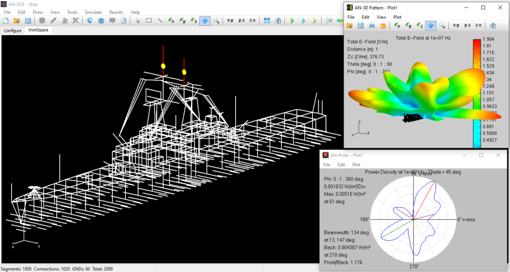
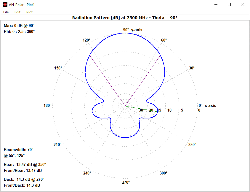
In the far-field zone, situated several wavelengths away from the structure, the magnetic field becomes proportional to the electric field. As a result, the electric field intensities are commonly used to analyze the results. This region is depicted in polar diagrams, as illustrated in Fig. 6, where the radiated field is represented as a function of direction. A more comprehensive representation can be achieved by plotting a 3D pattern, where radiation lobes can be superimposed onto the structure’s geometry, providing enhanced visualization of its directional properties, as exemplified in Fig. 7.

AN-SOF stands out as the easiest-to-use software tool for simulating antennas, particularly those that can be modeled using conductive wires. Are you ready to embark on your first simulation? Let’s get started!

Explore Our Pre-Computed Examples in the Models Tab

AN-SOF includes a collection of pre-calculated models that enable users to quickly load example projects directly into the interface. These models are organized into categories for easy navigation, making this feature especially useful for users exploring example designs and learning key antenna concepts.

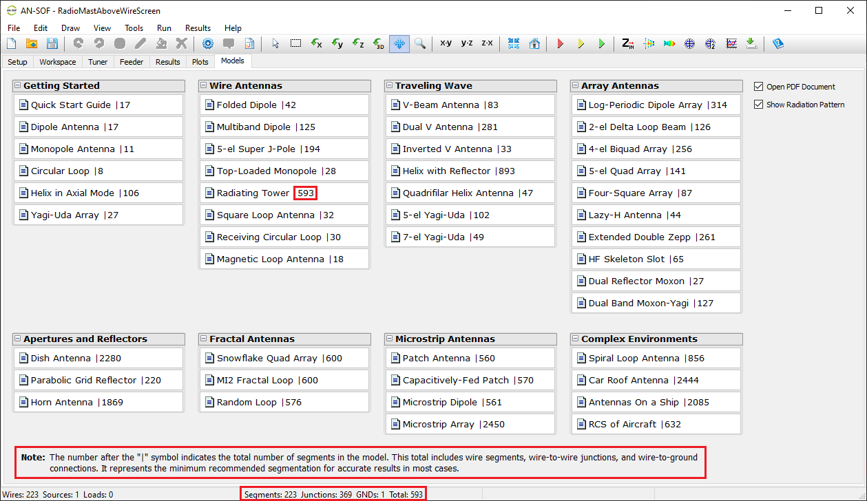
In the Models tab, you’ll find quick-access buttons for opening example models (see Fig. 8). Each model displays a 3D radiation pattern and includes a PDF guide with informational resources. Since all models are pre-calculated, they can be opened and explored using the AN-SOF Trial version.

Please note that the AN-SOF Trial version supports models with up to 50 segments plus connections. If you modify an example model and it exceeds this limit, you will need an active license for the AN-SOF PRO Edition to re-run simulations.

To explore the example models, simply click the buttons in the Models tab. On the right side of the screen, you can use the options “Open PDF Document” and “Show Radiation Pattern” to toggle the display of the PDF guide or the radiation pattern plot as needed.

Performing the First Simulation with AN-SOF

Several example files are included in the AN-SOF installation directory, located within a folder named “Examples”. When opening a file with the extension “.emm”, the wire structure will be displayed on the screen. To run the calculation, click on the Run ALL button on the toolbar. The main results can be plotted by clicking on the following buttons: Plot Current Distribution, Far-Field 3D Plot, and Far-Field Polar 1 Slice.

As a first experience using AN-SOF, let’s simulate a standard half-wave dipole, which is one of the simplest antennas that can be modeled. A dipole is a straight wire that is fed at its center. When the wire’s cross-section is circular, it is referred to as a cylindrical antenna. Since the wire is typically made of a highly conductive material, it can be considered a perfect conductor with zero resistivity. Therefore, we will model a cylindrical antenna with zero resistivity in this example. Follow the steps below to perform this simulation.

Step 1: Setup

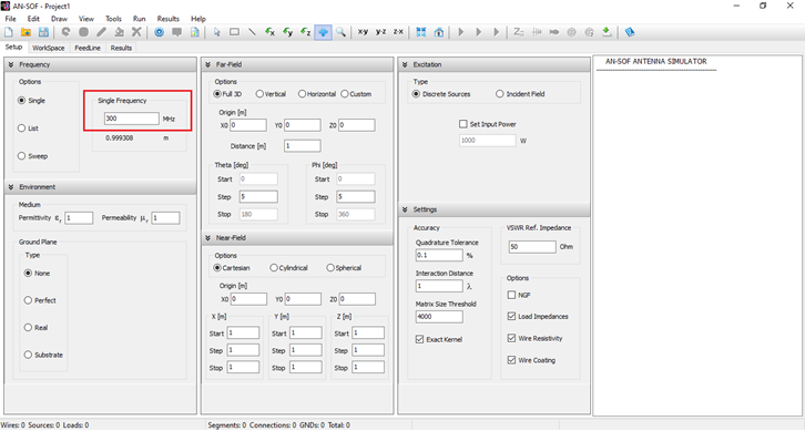
The first step is to set the operating frequency. Navigate to the Setup tab in the AN-SOF main window. Within the Frequency panel, there are three options to choose from. Select Single and enter the operating frequency for the antenna (see Fig. 9). In this case, the frequency is given in megahertz (MHz), and lengths are measured in meters (m). If desired, you can change the unit system for frequencies and lengths by going to Tools > Preferences. Please note that for a frequency of 300 MHz, the wavelength is approximately 1 meter (0.999308 m).

Step 2: Draw

Once the operating frequency has been set, you can draw the antenna geometry on the Workspace tab. The workspace is where the wire structure is visualized, representing a 3D space that allows zooming, rotation, and movement.

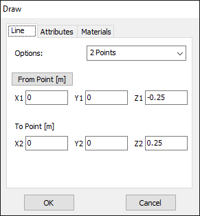
In AN-SOF, a straight wire is referred to as a Line. To draw a line, go to the main menu and select Draw > Line. This will open the Draw dialog box. In the Line tab, you can set the coordinates of two distinct points.

For this example, we will create a line along the z-axis that is 0.5 meters long, corresponding to half a wavelength at 300 MHz. Figure 10 illustrates the chosen starting point of the line at (X1, Y1, Z1) = (0, 0, -0.25) m, and the ending point at (X2, Y2, Z2) = (0, 0, 0.25) m. Next, switch to the Attributes tab (see Fig. 11). To ensure accurate results, the line should be divided into segments that are relatively short compared to the wavelength. Generally, a segment length equal to or less than one-tenth of a wavelength is considered short. AN-SOF suggests a minimum number of segments to achieve reliable results automatically. If you require higher resolution, you can increase the number of segments.

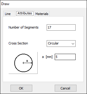
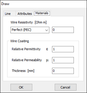
In this case, the line will be divided into 17 segments, and the wire cross-section will be circular with a radius of 5 millimeters. On the Materials tab (refer to Fig. 12), you can set the wire’s resistivity to zero.

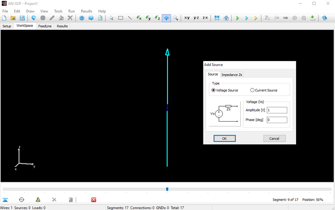
The next step is to feed the dipole. Right-click on the wire and select the Source/Load command from the pop-up menu that appears. A toolbar with a slider will be displayed at the bottom of the screen. Move the slider to the segment located at the center of the wire. Then, click the Add Source button. Add a voltage source with an amplitude of 1 Volt and a phase of zero (see Fig. 13).

Step 3: Run

To run the calculation, go to Run > Run Currents in the main menu. Once the calculations are completed, proceed to Run > Run Far-Field in the main menu. This will calculate the current distribution on the dipole antenna and the radiated field.

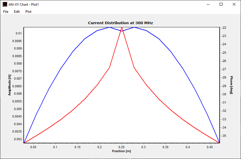
AN-SOF provides integrated graphical tools for result visualization. Right-click on the wire and select Plot Currents from the displayed pop-up menu. A plot showing the current distribution in amplitude along the dipole antenna will be displayed (refer to Fig. 14). Since a half-wave dipole has been drawn, the resulting current distribution resembles a semi-cycle approaching a sine function.

You can obtain several parameters from the perspective of the voltage source connected to the antenna terminals. Right-click on the wire and select List Currents from the pop-up menu. Move the slider to the position of the voltage source and click on the Input List button. This will display the input impedance of the dipole antenna, along with many other parameters (see Fig. 15).

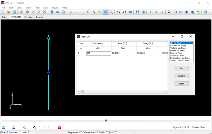
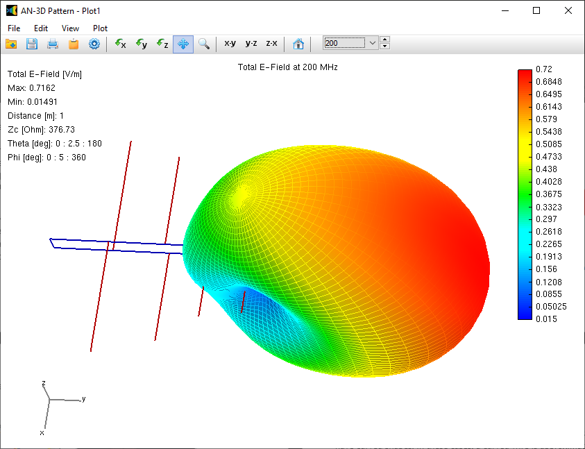
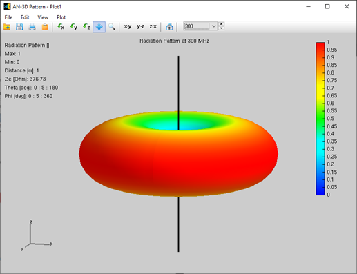
Alternatively, you can obtain the input impedance by simply clicking on the List Input Impedances (Zin) button in the main toolbar. To represent the radiation pattern in a 3D plot, navigate to Results > Plot Far-Field Pattern > 3D Plot in the main menu. The normalized radiation pattern will be displayed in the AN-3D Pattern application. A color bar-scale indicates the field intensities over the radiation lobes. Additionally, you can plot the directivity, gain, and electric field patterns by accessing the Plot menu in AN-3D Pattern. In the case of a half-wave dipole, it exhibits omnidirectional characteristics in the plane perpendicular to the dipole axis (xy-plane) (refer to Fig. 16).

As you have just experienced, a simulation consists of three simple steps. We hope you have enjoyed this example. For additional step-by-step examples, please visit our section titled Examples > Step by Step.

Summary

The key advantages of AN-SOF can be summarized as follows:

• AN-SOF is antenna modeling and design software that offers fast and user-friendly input and output graphical interfaces.

• AN-SOF employs the Conformal Method of Moments with Exact Kernel, resulting in enhanced accuracy and speed.

• AN-SOF provides an extended frequency range, enabling simulations from extremely low frequencies (such as 60 Hz circuits) to microwave antennas.

Simulating a wire structure involves a three-step procedure:

1. Setup: Set frequencies, environment, and desired results.

2. Draw: Draw the geometry, specify materials, and add sources.

3. Run: Perform the calculation and visualize the results.

At the beginning of the simulation, you can choose a convenient unit system for frequencies and lengths. This choice can be adjusted later by accessing Tools > Preferences. For instance, wire lengths are typically measured in meters (m) or feet (ft) for frequencies below 100 MHz, while millimeters (mm) or inches (in) are commonly used for higher frequencies.