Monopole Antennas Over Imperfect Ground: Modeling and Analysis with AN-SOF

Created OnOctober 17, 2022

Updated OnFebruary 12, 2025

By:Tony Golden

Explore the design and simulation of monopole antennas over imperfect ground using AN-SOF. Learn how ground conditions impact performance and optimize efficiency for LF/MF broadcasting applications.

Monopole antenna model (left), 3D radiation pattern in linear scale (top right), and 3D radiation pattern in decibel scale (bottom right).

Introduction

A monopole antenna is a class of radio antenna consisting of a single radiating element, typically mounted vertically over a conductive ground plane. It is one of the simplest and most widely used antenna designs, particularly in applications where space and simplicity are critical. The monopole can be thought of as half of a dipole antenna: by introducing a ground plane, one of the dipole’s two radiating elements is effectively replaced by the ground plane’s mirror image, creating a virtual “second leg.” This results in a structure that is electrically equivalent to a dipole but requires only half the physical height, making monopoles particularly advantageous for low-frequency and compact installations.

Monopole antennas are commonly used in a variety of applications, including AM/FM broadcasting, LF (Low Frequency) and MF (Medium Frequency) communication systems, mobile and base station antennas, and amateur radio setups. Their omnidirectional radiation pattern in the horizontal plane makes them ideal for broadcasting and communication over wide areas. However, their performance is highly dependent on the quality of the ground plane, as losses in the ground can significantly reduce efficiency and gain.In this article, we will simulate a monopole antenna in the form of a radio mast operating over imperfect ground, typical of LF and MF broadcasting scenarios. We will explore the impact of ground conditions on antenna performance and demonstrate how to optimize the design for improved efficiency.

Step 1 | Setup

Navigate to the Setup tab and set the operating frequency to 3 MHz in the Frequency panel. Next, go to the Environment panel > Ground Plane box and select the Real option, as shown in Fig. 1. Choose the Radial wire ground screen and Poor ground options. Note that the soil conductivity will automatically be set to 0.001 S/m and the relative permittivity (dielectric constant) to 5.

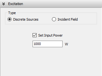
Finally, configure the number of radials, their length, and their radius as illustrated in Fig. 1. For radio masts, it is common practice to use a constant input power as a reference, such as 1 kW. Proceed to the Excitation panel, select Discrete Sources, then choose Set Input Power and enter 1,000 W, as shown in Fig. 2.

*Fig. 1: Configuring a radial wire ground screen in the Environment panel of AN-SOF.*

*Fig. 2: Configuring discrete sources in the Excitation panel with an input power of 1,000 W.*

Step 2 | Draw

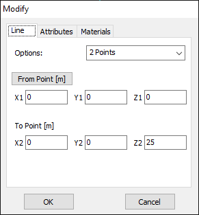
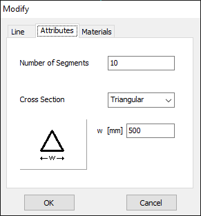
Right-click on the workspace and select Line from the pop-up menu. Specify a vertical wire with a height of 25 meters (equivalent to 1/4 wavelength at 3 MHz) and a triangular cross-section, as illustrated in Fig. 3. Although the recommended minimum number of segments is 3, we will divide the wire into 10 segments to achieve higher resolution in the current distribution. Note that the wire will automatically be connected to the ground at the origin (0, 0, 0).

Next, right-click on the wire and select the Source/Load command from the pop-up menu. Place a voltage source on the first segment to ensure the source is connected to the base of the mast. For further details, refer to the Adding Sources section.

*Fig. 3(a): Defining a vertical wire in the Line configuration page.*

*Fig. 3(b): Configuring a triangular cross-section in the Attributes page.*

Step 3 | Run

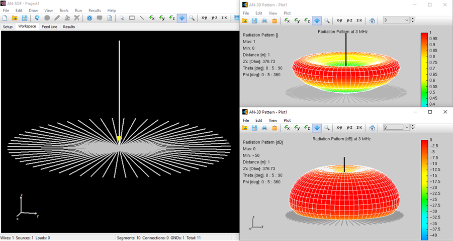
Click on the Run Currents and Far-Field (F11) button located on the toolbar. Once the calculations are complete, click on the Far-Field 3D Plot button on the toolbar to display the radiation pattern. In the AN-3D Pattern window, select Radiation Pattern from the Plot menu to generate the normalized radiation pattern (dimensionless). Then, choose the Radiation Pattern [dB] option to view the pattern in decibel scale. Note that the far field exhibits a null on the xy-plane due to losses in the ground plane, as shown in Fig. 4.

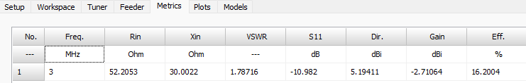
The antenna efficiency is defined as the ratio of radiated power to input power. Navigate to the Results tab to view key parameters such as input impedance, VSWR, directivity, gain, and efficiency, as illustrated in Fig. 5. You will observe that the efficiency is relatively low, which consequently results in low gain, as a significant portion of the input power is dissipated in the ground. In this example, we have intentionally chosen a Poor soil condition. To improve antenna efficiency, experiment with different soil types, increase the number of radial wires, and adjust their lengths.

Download Model

*Fig. 5: Results tab displaying input impedance and radiation parameters for the quarter-wave monopole antenna over a radial wire ground screen.*

Conclusion

Simulating monopole antennas using the AN-SOF Antenna Simulator offers significant advantages for engineers and designers. By leveraging its advanced modeling capabilities, users can accurately predict antenna performance, optimize designs, and evaluate the impact of various ground conditions without the need for costly and time-consuming physical prototypes.

The ability to analyze parameters such as radiation patterns, input impedance, gain, and efficiency provides invaluable insights, enabling the development of high-performance monopole antennas tailored to specific applications.

Whether you’re designing for LF/MF broadcasting, mobile communications, or amateur radio, AN-SOF empowers you to explore design trade-offs and achieve optimal results with precision and efficiency.