Plotting Near Field Patterns

In AN-SOF, near-field analysis allows you to evaluate the electric ($\mathbf{E}$) and magnetic ($\mathbf{H}$) fields in the immediate vicinity of an antenna or at any specified distance. This is essential for studying antenna-to-antenna coupling or electromagnetic compatibility (EMC).

Defining the Calculation Grid

Before plotting, you must define the observation points in the Near-Field panel of the Setup tab. You can specify the grid using:

• Cartesian Coordinates (X, Y, Z)
• Cylindrical Coordinates (R, Phi, Z)
• Spherical Coordinates (R, Theta, Phi)

Verification in the Far-Field

While these are “near-field” tools, they can be used to verify far-field behavior. As you move further from the antenna, you should observe:

1. $\mathbf{E}$ and $\mathbf{H}$ becoming perpendicular to each other and the radial direction.
2. Fields oscillating in phase.
3. The intrinsic impedance of free space: $|\mathbf{E}| / |\mathbf{H}| \approx 120\pi\ \Omega \approx 377\ \Omega$.

Power Density and Compliance

If both $\mathbf{E}$ and $\mathbf{H}$ fields are calculated, AN-SOF provides the RMS Power Density ($S$), calculated as:

$S \,=\, |\mathbf{E} \times \mathbf{H}^*|$

This metric is critical for ensuring that your design complies with human exposure limits (e.g., ICNIRP or FCC standards).

3D Visualization

To visualize the fields as a 3D color-coded map, use the following paths in the main menu:

• Electric Field: Results > Plot Near E-Field Pattern > 3D Plot
• Magnetic Field: Results > Plot Near H-Field Pattern > 3D Plot
• Power Density: Results > Plot Power Density Pattern > 3D Plot

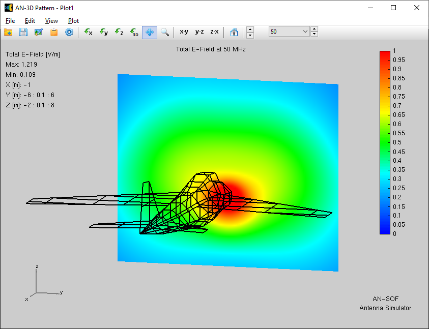
These commands launch AN-3D Pattern (Fig. 1). If your simulation includes multiple frequencies, you will be prompted to select a specific frequency before the plot is rendered.

2D Visualization and Individual Components

For a more detailed look at field gradients along a specific axis or path, use the 2D Plot options under the same Results menus. This launches AN-XY Chart.

• Total RMS: The default view shows the total magnitude.
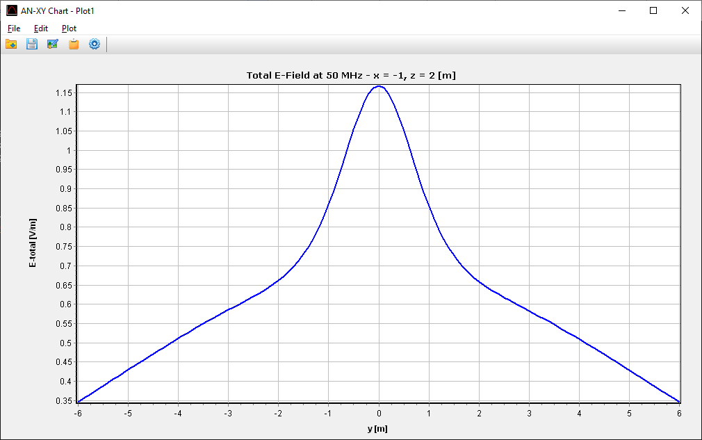
• Individual Components: You can isolate specific vectors (e.g., $E_x, E_y, E_z$) by navigating to the Plot menu within AN-XY Chart (Fig. 2).

Tabulating and Exporting Data

To see the exact numerical values at every grid point, use:

• Results > List Near E-Field Pattern
• Results > List Near H-Field Pattern
• Results > List Power Density Pattern

These tables can be exported for further analysis in external mathematical tools.

Understanding Field Components by Coordinate System

The components of the electric and magnetic fields calculated by AN-SOF depend entirely on the coordinate system you select in the Near-Field panel of the Setup tab. Choosing the right system is crucial for matching the grid to the physical symmetry of your antenna.

1. Cartesian Coordinates $(x, y, z)$

When you select a rectangular grid, the fields are decomposed into their standard orthogonal components. This is ideal for planar structures or when evaluating fields along a straight line or over a flat surface.

• Electric Field Components: $E_x, E_y, E_z$
• Magnetic Field Components: $H_x, H_y, H_z$

2. Cylindrical Coordinates $(\rho, \phi, z)$

This system is best suited for structures with axial symmetry, such as vertical monopoles or circular arrays. The components are calculated relative to the radial distance from the $z$-axis and the rotation around it.

• Electric Field Components: $E_\rho$ (radial), $E_\phi$ (azimuthal), $E_z$ (axial)
• Magnetic Field Components: $H_\rho, H_\phi, H_z$

3. Spherical Coordinates $(r, \theta, \phi)$

Spherical coordinates are typically used to analyze how fields radiate outward into space. This setup is perfect for visualizing how near-fields begin to transition into far-field patterns.

• Electric Field Components: $E_r$ (radial), $E_\theta$ (zenith/elevation), $E_\phi$ (azimuth)
• Magnetic Field Components: $H_r, H_\theta, H_\phi$

Tip

In the AN-XY Chart application, you can isolate these individual components via the Plot menu to see which specific orientation contributes most to the total field magnitude at a given point.