Search for answers or browse our Knowledge Base.
Guides | Models | Validation | Book
Numerical Convergence and Stability of Input Impedance in Cylindrical Dipoles
Examine the numerical stability of cylindrical dipole modeling through this rigorous convergence study. By analyzing input impedance as a function of discretization density and length-to-radius ratios, this article demonstrates how AN-SOF overcomes the traditional divergence issues found in many MoM codes, such as NEC-2. While older engines often fail to provide convergent reactance values when using a delta-gap source with fine segments, AN-SOF’s exact kernel ensures monotonic stability. Validation against the classical 73.1 + j 42.5 Ohm half-wave dipole thin-wire limit and convergence analysis confirm the engine’s precision for both resonant and anti-resonant linear antennas.
Introduction to Discretization and Convergence
A fundamental validation check for any computational electromagnetics (CEM) solver involves incrementing the number of segments used to model an antenna while keeping the physical dimensions (length, radius, and source gap) constant. Under these conditions, the calculated input impedance ($Z_{\text{in}}$) should converge toward a stable asymptotic value. This process ensures that the numerical results are not arbitrary artifacts of the mesh density but are instead reliable representations of the underlying physics.
However, calculating input impedance is a highly sensitive task, particularly regarding the modeling of the source excitation. Most Method of Moments (MoM) codes utilize a delta-gap source model, which can lead to numerical instability if the solver formulation is not sufficiently robust. This article examines the stability of the AN-SOF engine, focusing on its ability to produce convergent results across various electrical lengths and wire thicknesses.
The Delta-Gap Source Challenge: AN-SOF vs. NEC-2
One of the most significant challenges in wire antenna modeling is the behavior of the input impedance as the segment length at the source position decreases. In many traditional engines, such as the widely used NEC-2 (Numerical Electromagnetics Code), the input impedance (particularly the reactive component) tends to diverge as the discretization becomes finer.
This divergence occurs because as the number of segments increases, the length of the segment where the delta-gap voltage is applied tends toward zero. In codes that rely on certain thin-wire approximations or integral equation kernels that do not adequately handle the near-field singularity of the source, this leads to unstable results.
In contrast, the AN-SOF results remain remarkably stable. As shown in the simulation data, the input impedance in AN-SOF grows monotonically and stabilizes even as the segments become extremely small. This stability is a direct result of the exact kernel implementation in AN-SOF, which accurately computes the potential integrals even in the immediate vicinity of the source. This ensures that the reactance converges to a physically meaningful value, providing a significant advantage over NEC-type solvers for precision impedance matching.
Convergence Profiles and Electrical Length
To evaluate these stability characteristics, the input impedance was simulated as a function of the number of segments ($N$) in each arm of a dipole antenna of half-length $h$ and radius $a$, as shown in Fig. 1. Both dimensions are normalized to the operating wavelength $\lambda$.
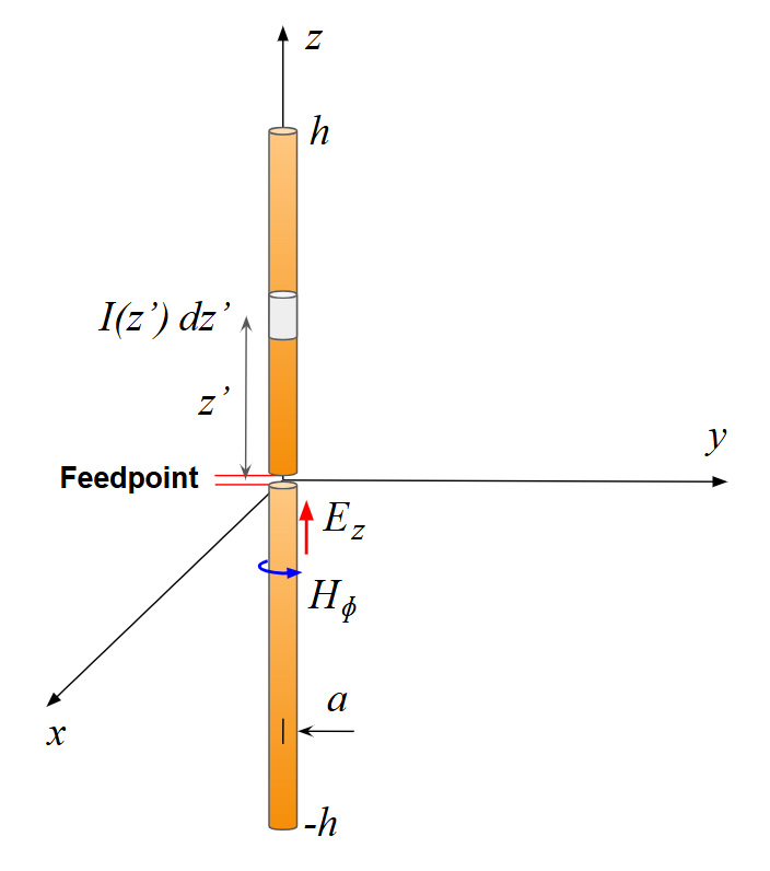
Figure 2 illustrates these results for three distinct electrical lengths:
- Short Dipole ($h/\lambda = 0.175$): Characterized by high capacitive reactance.
- Half-Wave Dipole ($h/\lambda = 0.25$): The primary length just above the first series resonance.
- Full-Wave Dipole ($h/\lambda = 0.5$): The high-impedance anti-resonant state.
These parameters were tested for two wire radii: a thin wire ($a/\lambda = 0.001191$, equivalent to $a = 3/32″$ at $\lambda = 1 \text{ m}$) and a thicker conductor ($a/\lambda = 0.009525$, equivalent to $a = 3/4″$ at $\lambda = 1 \text{ m}$). The results in Fig. 2 confirm that AN-SOF provides a smooth, monotonic approach to the asymptotic impedance value for both input resistance ($R$) and reactance ($X$). This stability across different radii and electrical lengths demonstrates that the engine is not limited by wire thickness or the operating mode of the antenna.
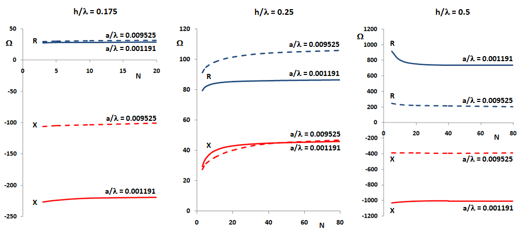
In practice, these curves demonstrate that using 20 segments per wavelength along a linear antenna results in an input impedance within approximately 5% of its asymptotic value. Even with 10 segments per wavelength, the error remains between 10% and 15%, which is sufficient for a first approximation.
We can also investigate the convergence behavior of the input impedance of a center-fed cylindrical antenna of fixed dimensions as a function of frequency. Figure 3 shows the input resistance and reactance spectrum of a dipole with a length of $2h = 0.5 \text{ m}$, a radius of $a = 5 \text{ mm}$, and a feed gap of $0.02 \text{ m}$. As the frequency varies from $100$ to $1500 \text{ MHz}$, the wavelength ranges from $0.2 \text{ m}$ to $3 \text{ m}$. Consequently, the normalized antenna dimensions vary across the following ranges:
$0.167\lambda < 2h < 2.5\lambda \text{,}$
$0.00167\lambda < a < 0.025\lambda \text{,}$
$0.00667\lambda < \text{gap} < 0.1\lambda \text{.}$
Three curves were obtained for $N = 5$, $10$, and $20$ segments in each antenna arm.
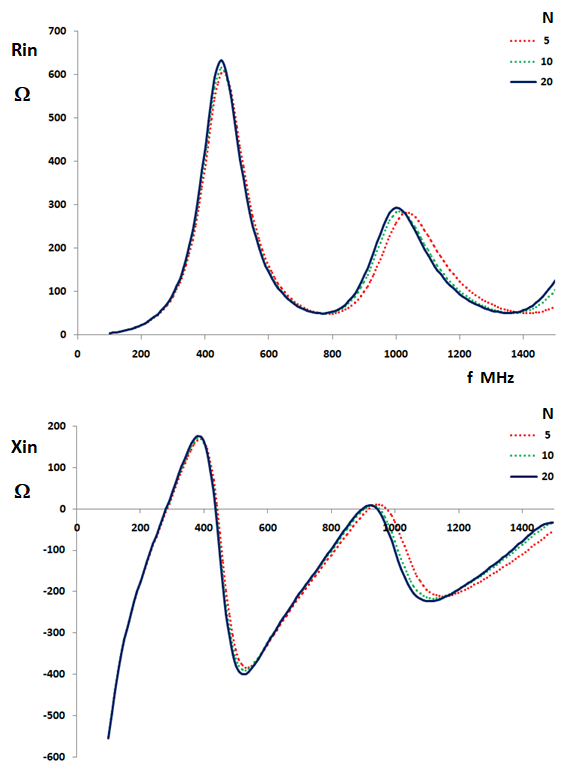
We can see that the input impedance curves converge toward a single curve as the number of segments increases. Furthermore, the difference between the curves for $N = 10$ and $N = 20$ remains small even at frequencies as high as $1200 \text{ MHz}$, corresponding to a wavelength of $\lambda = 0.25 \text{ m}$ and a dipole length of $2\lambda$.
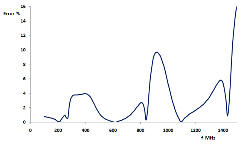
This result reinforces the previous recommendation of using 10 segments per wavelength ($2N/2\lambda$ for $N = 10$) to obtain practically useful values for the input impedance. Figure 4 shows the percentage difference between the absolute values of the input impedance for $N = 10$ and $N = 20$, with the error staying well below 5% across most of the analyzed frequency range. Only near the third resonance, at approximately $900 \text{ MHz}$, does the error rise to 10%. Additionally, the useful bandwidth for the 10-segments-per-wavelength rule extends to $1450 \text{ MHz}$ ($\lambda = 0.207 \text{ m}$), where the dipole length is $0.5 \text{ m} / 0.207 \text{ m} = 2.4\lambda$. This suggests that even 8 segments per wavelength ($2N/2.4\lambda$ for $N = 10$) can provide acceptable results.
Comparison with NEC-2 Results
A comparative analysis between AN-SOF and the legacy NEC-2 engine reveals significant differences in numerical stability. In Fig. 5 (left), the input impedance of a center-fed half-wave dipole is plotted as a function of the number of segments ($N$) in each arm, using a radius of $0.005\lambda$ and a source gap of $0.025\lambda$. While the results obtained from AN-SOF converge monotonically, the NEC-2 results exhibit clear divergence.
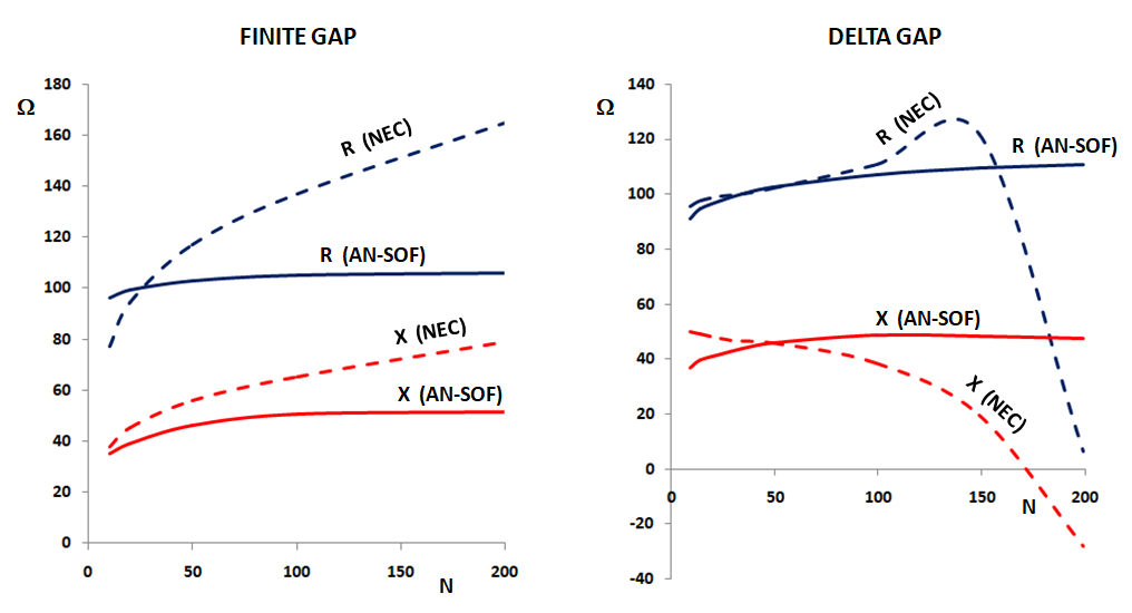
The divergence observed in the NEC-2 impedance calculations stems from two primary factors. First, as discretization increases, a disparity grows between the fixed width of the source gap and the decreasing length of the adjacent segments. Because the gap is filled by a single segment, the model eventually connects segments of significantly different lengths. This is a known limitation of the NEC-2 architecture, which requires connected segments to maintain comparable lengths to ensure numerical accuracy.
Second, as the number of segments increases, each segment becomes shorter relative to its radius. In these cases, the radius-to-length ratio increases, effectively making the segments “thick.” While NEC-2 utilizes an extended kernel to approximate thick-wire behavior, it lacks the exact kernel necessary to handle the complex near-field interactions of these geometry-constrained segments.
The kernel is the fundamental component of the integral equation solved via the Method of Moments (MoM) to determine current distribution. Many traditional MoM implementations rely on thin-wire or extended approximations of the kernel. AN-SOF avoids the instabilities associated with NEC-2 by utilizing an exact kernel. This formulation allows the solver to maintain high precision regardless of the radius-to-length ratio or variations in adjacent segment lengths. While rounding errors exist at extreme limits, they remain beyond the reach of standard practical simulations.
The stability of the exact kernel is further demonstrated in Fig. 5 (right) using a delta-gap source model. In this configuration, the gap width effectively tends toward zero, meaning the segment at the source position continuously decreases in length as the mesh is refined. Although the delta-gap model is theoretically known to cause impedance divergence in numerical solvers, the AN-SOF results remain stable and grow monotonically. In fact, the reactance achieves a state of near-convergence, providing a reliable and predictable result that stands in stark contrast to the instability of legacy engines.
The Thin-Wire Asymptotic Limit
A classic benchmark in electromagnetic theory is the input impedance of a half-wave dipole as its radius approaches zero. Theoretically, for an infinitely thin antenna, the input impedance reaches a limit of $73.1 + j 42.5\ \Omega$. This provides a definitive horizontal asymptote for validating numerical precision.
Figure 6 shows the AN-SOF results for the input impedance of a center-fed half-wave dipole plotted against the length-to-radius ratio ($2h/a$). The simulation sweep covers an extensive range from $10^2$ to $10^6$. As the $2h/a$ ratio increases (representing an increasingly thin wire), the calculated resistance and reactance converge seamlessly toward the theoretical $73.1\ \Omega$ and $42.5\ \Omega$ benchmarks.
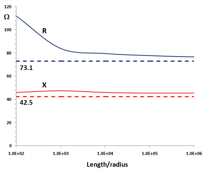
An important observation from Fig. 6 is the role of the source gap. While the gap width was maintained at $0.0025\lambda$, the input impedance becomes increasingly independent of the gap width as the length-to-radius ratio grows. This decoupling is a desirable trait in a solver, as it indicates that the fundamental resonant behavior of the antenna is being captured correctly without excessive sensitivity to the specific physical dimensions of the feed-point gap.
Conclusions
The convergence analysis of the cylindrical dipole validates several key technical strengths of the AN-SOF engine:
- Robustness Against Source Divergence: Unlike NEC-2 and similar codes where the delta-gap source can cause impedance divergence, AN-SOF provides stable, monotonically growing results. This is critical for engineers and designers who must use fine discretization to model complex structures without sacrificing the accuracy of the feed-point parameters.
- Theoretical Precision: The alignment with the $73.1 + j42.5\ \Omega$ thin-wire limit (Fig. 6) confirms that the exact kernel implementation is mathematically sound and perfectly consistent with classical antenna theory.
- Reliability Across Resonances: The stable convergence observed for short, half-wave, and full-wave dipoles (Fig. 2) ensures that the solver is equally reliable for high-reactance sensors, standard resonant radiators, and high-impedance anti-resonant elements.
- Discretization Confidence: By demonstrating that results stabilize quickly as the number of segments increases, AN-SOF allows designers to achieve high-precision impedance results with efficient computational overhead.
Ultimately, these findings establish AN-SOF as a superior tool for impedance characterization. By successfully mitigating the numerical instability associated with the delta-gap source, the software provides a level of design confidence that traditional thin-wire approximation codes cannot match.
See Also:
Technical Keywords: Input Impedance Convergence, Numerical Stability, AN-SOF vs. NEC-2, Exact Kernel, Method of Moments (MoM), Delta-gap Source, Cylindrical Dipole, Discretization Density, Thin-wire Approximation, Monotonic Convergence.
