Modeling Lumped Loads in AN-SOF: Canceling Feedpoint Reactance for a Perfect Match

Don’t let a stubborn reactance stand between you and a perfect match. Whether your antenna is electrically long or short, this article provides a step-by-step guide to canceling the antenna feedpoint reactance using a lumped impedance. Through practical case studies on a 20m dipole and 40m vertical, learn how to use the 2-segment bridge method to model loading coils and series capacitors with pro-grade accuracy.

Introduction

Every ham knows the feeling: you’ve built a great antenna and reached the perfect height, but your analyzer shows a stubborn reactance ($X_{\text{in}}$) that prevents your VSWR from hitting that glorious 1:1. While “trimming the wire” is the classic fix, geometry or environmental constraints often make it impossible. In these cases, we turn to lumped components (inductors and capacitors) to cancel out the reactive part of the impedance. This guide demonstrates how to model that process accurately in AN-SOF.

The Goal: Reactance Cancellation

To achieve resonance, the total reactance at the feedpoint must be zero. This is accomplished by adding an equal and opposite reactance in series with the source:

1. If $X_{\text{in}} > 0$ (Inductive): The antenna is “electrically long,” requiring a series capacitor to cancel the reactance:

$\displaystyle C \,=\, \frac{1}{2\pi f \, X_{\text{in}}}$

2. If $X_{\text{in}} < 0$ (Capacitive): The antenna is “electrically short,” requiring a series inductor (loading coil) to cancel the reactance:

$\displaystyle L \,=\, -\, \frac{X_{\text{in}}}{2\pi f}$

In the preceding equations, $C$ represents the capacitance in Farads (F), $L$ denotes the inductance in Henries (H), $X_{\text{in}}$ is the antenna input reactance in Ohms ($\Omega$), and $f$ is the operating frequency in Hertz (Hz).

You can access a reactance to inductance and capacitance converter, as well as the reverse calculator, at the following link:

• 📐 RF Calculators

Modeling the “Tuning Bridge” in AN-SOF

To achieve the most accurate simulation, avoid simply “stacking” a load onto your source segment. Instead, model the physical gap that exists between your antenna terminals using the 2-Segment Method:

1. Leave a gap: In your antenna geometry, leave a space equal to the actual distance between your feedpoint terminals.
2. Draw a bridge: Create a short wire to span this gap.
3. Discretize the wire: Divide this short bridge wire into exactly two segments.
4. Assign components: Place the Discrete Source on the first segment and the Lumped Load (the $L$ or $C$) on the second.

This configuration is illustrated in Fig. 1, which demonstrates how to bridge the terminals of a simple dipole and assign a voltage source and load to the specific segments.

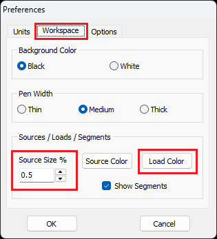
Because the bridge wire is typically very small relative to the overall structure, you may need to adjust the source symbol size (represented by a yellow circle) in the AN-SOF workspace. Additionally, the lumped load is often easier to visualize if assigned a high-contrast color, such as red. To adjust the source symbol size (e.g., setting it manually to 0.5%) and customize the load impedance color, navigate to Tools > Preferences > Workspace in the main menu (Fig. 2).

Case Study 1: The “Long” 20m Dipole

Consider a 10.6 m dipole constructed from AWG 14 copper wire (radius = 0.815 mm). The environment is free space, which serves as a baseline for verifying antenna performance before introducing ground effects. At 14.2 MHz, an AN-SOF simulation utilizing a 5 cm feedpoint gap yields the following input impedance:

$Z_{\text{in}} \,=\, 80 \,+\, j48\ \Omega$

Since $X_{\text{in}} = +48\ \Omega$, the antenna is electrically long. To achieve resonance, we calculate the required series capacitance as follows:

$\displaystyle C \,=\, \frac{1}{2\pi (14.2 \times 10^6)(48)} \,\approx\, 233.5\ \text{pF}$

The calculator below allows you to determine the capacitance in pF by entering the operating frequency in MHz and the required capacitive reactance:

Practical Implementation:

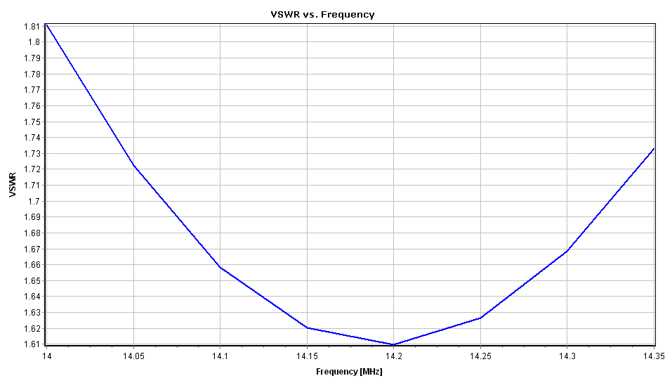
Since a precise 233.5 pF capacitor is difficult to source, a standard 220 pF or 240 pF high-voltage “doorknob” or silver mica capacitor should be used. Re-running the simulation in AN-SOF with a 220 pF capacitor (see Fig. 1) results in a 50-ohm VSWR of approximately 1.6:1. While not a perfect 1:1 match due to the $80\ \Omega$ input resistance, this remains well within the range of most internal rig tuners.

Figure 3 illustrates the 50-ohm VSWR across the 20m band (14.0 to 14.35 MHz) with the 220 pF capacitor installed. You can download the dipole model by clicking the button provided below the figure.

Case Study 2: The “Short” 40m Vertical

For a high-performance 40m vertical, we utilize 1-inch Aluminum tubing. This monopole antenna functions as a “half-dipole” in the air region, complemented by a radial wire ground screen (Fig. 4). The screen consists of 20 radials (AWG 12, 5 m long) installed over average ground (conductivity $\sigma = 0.005\text{ S/m}$, dielectric constant $\epsilon_r = 13$).

At 7.1 MHz, with a 10 cm feedpoint gap bridged by AWG 12 wire, AN-SOF reports:

$Z_{\text{in}} \,=\, 28 \,-\, j216\ \Omega$

With a reactance of $X_{\text{in}} = -216\ \Omega$, the antenna is electrically short and highly capacitive. To achieve resonance, a series loading coil (inductor) must be added at the feedpoint:

$\displaystyle L \,=\, -\,\frac{-216}{2\pi (7.1 \times 10^6)} \,\approx\, 4.84\ \mu\text{H}$

The following calculator allows you to determine the required inductance in $\mu\text{H}$ by entering the operating frequency and the capacitive reactance:

Practical Implementation:

A standard 4.7 $\mu$H inductor is an ideal choice for this application. In AN-SOF, you can model this by assigning 4.7 $\mu$H to the Lumped Load property of the second segment in your bridge wire.

The Resistance Match: 28 Ω to 50 Ω

Even after canceling the capacitive reactance, the radiation resistance ($R_{\text{in}}$) remains at 28 $\Omega$. On a standard $50\ \Omega$ coaxial line, this results in a 1.8:1 VSWR.

The Fix:

To lower the VSWR to a near-perfect 1.1:1, a 1:2 Impedance Ratio UnUn (Unbalanced-to-Unbalanced transformer) is required. This transforms the $28\ \Omega$ feedpoint to $56\ \Omega$, providing an excellent match for $50\ \Omega$ coax. A typical implementation uses a binocular ferrite core with a 5:7 turn ratio, yielding an impedance transformation of approximately 1.96.

Figure 5 shows the 50-ohm VSWR across the 40m band (7.0 to 7.3 MHz) with the 4.7 $\mu$H inductor installed. You can download the monopole antenna model by clicking the button below Fig. 4.

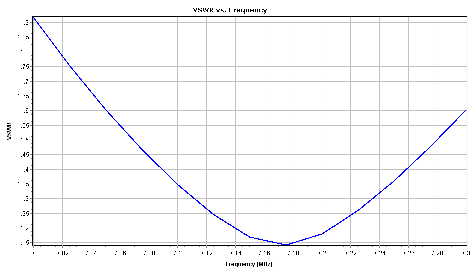
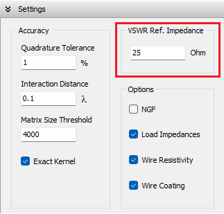
To simulate the effect of the 1:2 UnUn, navigate to the Setup tab > Settings panel and set the “VSWR Ref. Impedance” to $25\ \Omega$ before running the simulation (Fig. 6).

Simulation Tips

• Execution Optimization: Since the primary focus of these simulations is input impedance and VSWR, use the Ctrl + R shortcut to execute the current distribution calculation only. This avoids the unnecessary computational overhead of calculating the radiation pattern when it is not yet required. While users often default to Run Currents and Far-Field (F10) or Run ALL (F12), Ctrl + R is the most efficient choice for iterative impedance matching. The far-field or near-field metrics can be calculated separately via the Run menu once the matching network is finalized.

• Frequency-Dependent Reactance vs. Fixed Impedance: It is important to remember that the reactance of lumped components ($L$ or $C$) varies with frequency. Capacitive reactance is inversely proportional to frequency (decreasing as frequency increases), while inductive reactance is directly proportional (increasing as frequency increases). However, if the operating bandwidth is sufficiently narrow, the added reactance can be approximated as a constant. In such cases, you can set a fixed R + jX impedance in AN-SOF. For instance:
  • Case Study 1: Set $R = 0$ and $X = -48\ \Omega$.
  • Case Study 2: Set $R = 0$ and $X = 216\ \Omega$.

• This simplification allows for rapid antenna tuning, enabling you to move quickly to the analysis of far-field metrics, such as directivity and gain, before refining the physical components of the impedance matching system.

Conclusions

Achieving a perfect 1:1 VSWR often requires looking beyond physical wire dimensions and addressing feedpoint reactance directly. By calculating the necessary series inductance or capacitance, radio amateurs can effectively “electrically” tune an antenna that is otherwise constrained by geometry or environment.

The key to high-fidelity results in AN-SOF lies in the 2-segment bridge method, which accurately models the physical gap between antenna terminals and the integration of tuning components. While theoretical calculations provide a precise starting point, the use of standard, off-the-shelf components, and verifying their impact within the simulation, ensures that your real-world build performs as expected.

See Also:

• Complete Workflow: Modeling, Feeding, and Tuning a 20m Band Dipole Antenna

• Modeling a Center-Fed Cylindrical Antenna with AN-SOF

• Monopole Antennas Over Imperfect Ground: Modeling and Analysis with AN-SOF

Technical Keywords: Antenna Tuning, Reactance Cancellation, Lumped Loads, Input Impedance, VSWR, Loading Coil, Series Capacitor, 2-Segment Method, Feedpoint Gap, Antenna Resonance, 20m Dipole, 40m Vertical, Radial Wire Ground Screen, UnUn Transformer, Impedance Matching.

---