Antenna Far-Field Comparison using Multi-Slice and Multi-Frequency Plots

This guide explains how to leverage the advanced multi-slice and multi-frequency plotting capabilities of the AN-Polar application in AN-SOF (Version 11 and later). Learn how to compare antenna far-fields by overlaying up to five angular cuts or frequency steps in a single polar diagram, importing and exporting pattern data using .plr files to compare different designs, and optimizing coordinate scales for linear and logarithmic representations.

1. Introduction and Overview

From version 11 of AN-SOF, the AN-Polar application has the capability to plot up to five slices in a single polar diagram. This feature is highly valuable for conducting direct comparative analyses of different radiation patterns.

The plotted slices can represent:

• Angular cuts: Horizontal or vertical planes of a 3D radiation pattern.
• Multi-frequency steps: Patterns corresponding to different frequencies when a frequency sweep has been calculated.
• Different antenna designs: Overlaid polar radiation patterns imported from independent antenna simulation projects.

This guide provides a detailed technical walkthrough of how to configure, scale, and manage these multi-slice options to optimize your antenna analysis workflow.

2. Configuring Multi-Slice Polar Plots

To make polar slices available for plotting, a radiation pattern calculation must be completed previously in AN-SOF.

Step-by-Step Configuration:

1. Navigate to the main menu and select: Results > Far-Field Angular Plot > Multi-Slice Polar…
2. If a frequency sweep was performed, the software will prompt you to select the target frequency, as radiation patterns are frequency-dependent.
3. After selecting the frequency, the configuration dialog box shown in Fig. 1 will appear.
4. In the Cut Orientation panel, select either:
   • Fixed Theta (Horizontal slices, where the polar angle $\theta = \text{constant}$)
   • Fixed Phi (Vertical slices, where the azimuth angle $\phi = \text{constant}$)
5. Use the drop-down menus to assign values for Slices 1 to 5:
   • Slice 1 is mandatory and will always be plotted.
   • Slices 2 to 5 are optional. Enable them by checking their respective selection boxes.

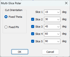
🗒️ Example (Fig. 1): With all five slices checked under a Fixed Theta orientation, we can plot the horizontal slices at $\theta = 15^\circ$ (Slice 1), $\theta = 30^\circ$ (Slice 2), $\theta = 45^\circ$ (Slice 3), $\theta = 60^\circ$ (Slice 4), and $\theta = 90^\circ$ (Slice 5, which corresponds directly to the physical $xy$-plane).

3. Scale Optimization and Polarization Controls

3.1. Logarithmic vs. Linear Coordinate Scales

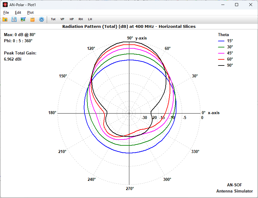
Figure 2 shows an example of five horizontal slices plotted for a Log-Periodic Dipole Array (LPDA) at $400\text{ MHz}$.

• Pattern Interpretation: The polar slices display diminishing maximum values as we transition from $\theta = 90^\circ$ to $\theta = 15^\circ$, reflecting that the maximum radiation intensity occurs on the $xy$-plane ($\theta = 90^\circ$).
• Peak Gain: The absolute peak total gain is displayed in the upper-left corner of the chart (e.g. $6.962\text{ dBi}$).
• Dynamic Range: The default scale ranges from a center value of $-100\text{ dB}$ to $0\text{ dB}$ at the outer circle, representing a normalized radiation pattern in decibels.
• ARRL-Style Log Scale: By default, AN-Polar utilizes a modified logarithmic scale (popularized by the ARRL) which compresses the center of the chart. This allows sidelobes and backlobes to remain visible without distorting the main lobe.

To switch from the logarithmic scale to a linear scale:

1. Navigate to Edit > Preferences in the AN-Polar main menu (or click the Gear icon on the toolbar).
2. Under the scale type options, choose Lin (Linear) instead of Log.
3. Adjust the dB Depth (the minimum value represented at the center of the plot, default $-100\text{ dB}$).

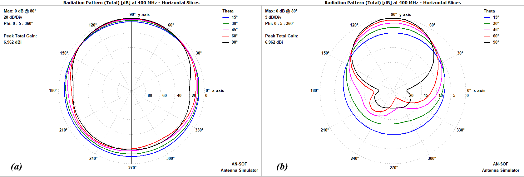
📝 Important Scaling Note: In a linear scale, small decibel differences are expanded near the center (e.g., $-50\text{ dB}$ sits exactly halfway between the center and the outer ring). To make the angular variations of a slice visually distinguishable for values above $-50\text{ dB}$, you must reduce the dB Depth to a narrower range, such as $-25\text{ dB}$.

Figure 3(a) and Figure 3(b) illustrate this effect, comparing a linear scale representation of the LPDA pattern with a dB depth of $-100\text{ dB}$ versus an optimized depth of $-25\text{ dB}$.

3.2. Non-Decibel Metrics

The linear scale is highly recommended when plotting dimensionless, non-logarithmic metrics. From the Plot menu, you can select:

• Directivity (dimensionless)
• Gain (dimensionless)
• Radiation Pattern (normalized to the range $0$ to $1$)

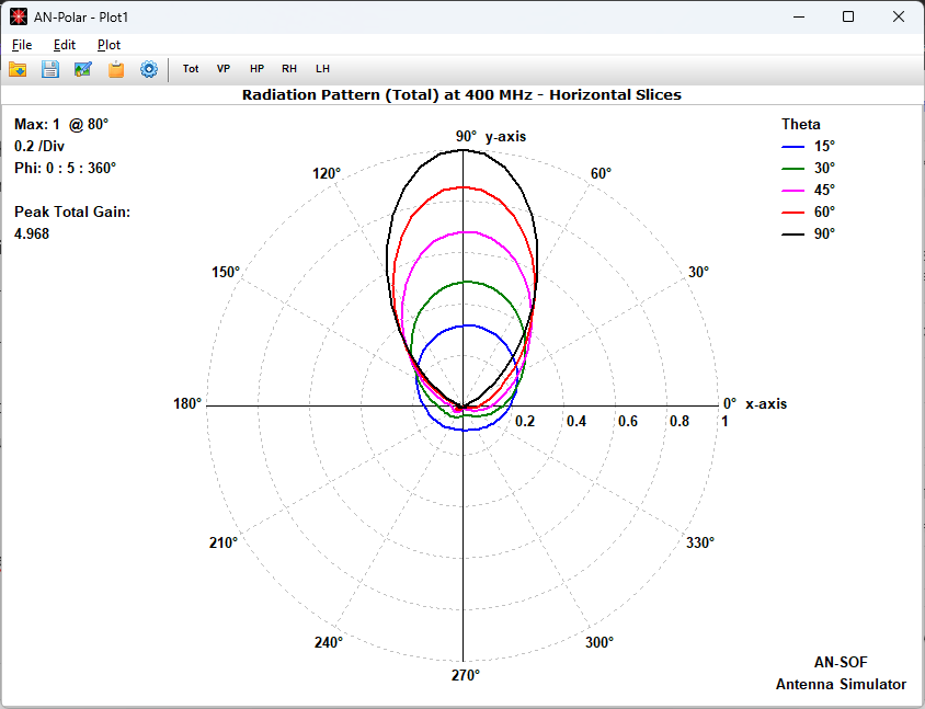
Figure 4 displays the normalized radiation pattern from Figure 2 in linear scale, where the center represents $0$ and the outer circle corresponds to $1$. Here, the peak total gain is shown as a dimensionless value of $4.968$. The logarithmic representation is derived using the standard formula:

$\displaystyle \text{Gain [dBi]} \,=\, 10 \, \log_{10}(4.968) \,\approx\, 6.962\text{ dBi}$

3.3. Polarization Controls

The AN-Polar toolbar includes quick-access buttons to instantly isolate specific polarization components of the computed far-field (Fig. 5):

• Tot (Total radiation pattern, directivity, gain, or E-field)
• VP (Vertically Polarized component)
• HP (Horizontally Polarized component)
• RH (Right-Hand Circularly Polarized component)
• LH (Left-Hand Circularly Polarized component)

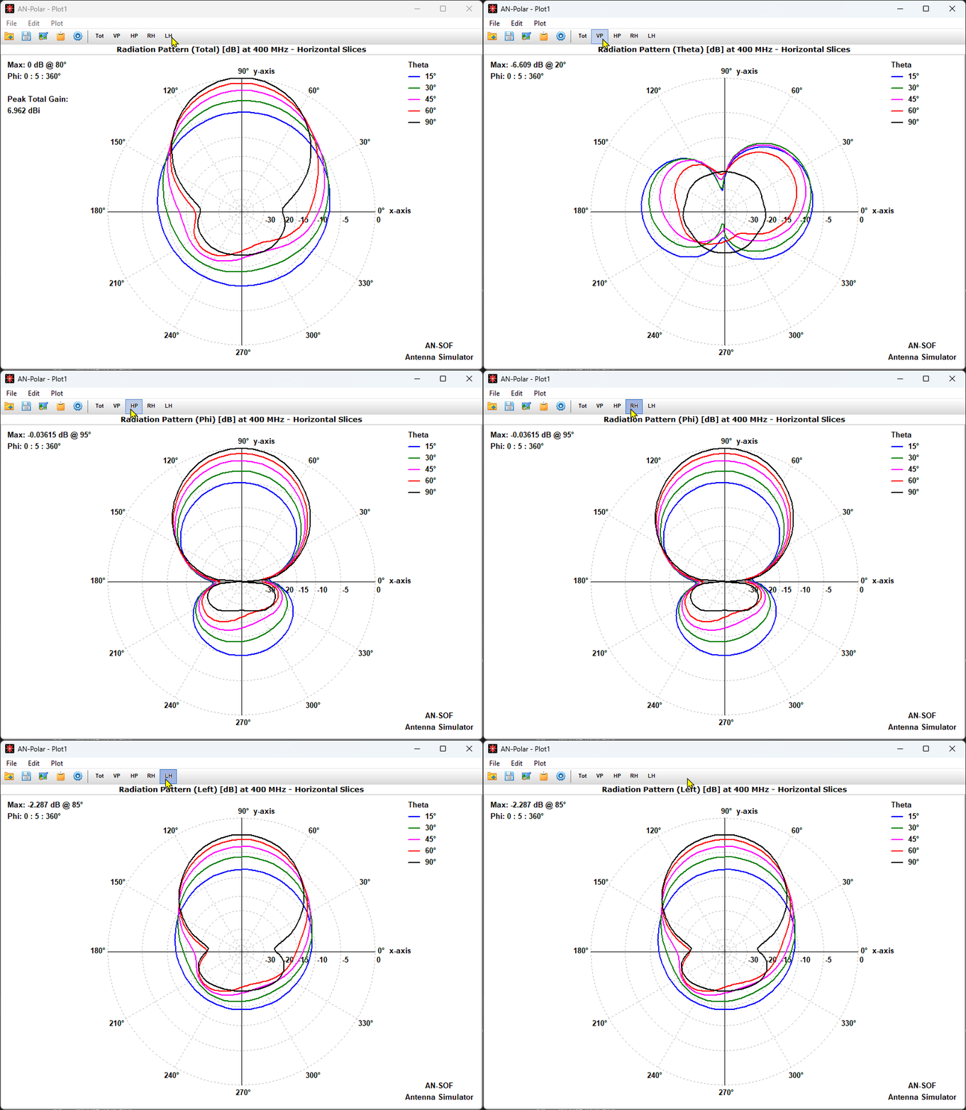
In the Plot menu the plotted metric can be changed, switching from radiation pattern, to power density, to gain, to directivity, to E-field, or to axial ratio.

📝 Important Scaling Note: The outer circle for each individual polarization component is automatically scaled and normalized independently. Consequently, this maximum boundary may not default to $0\text{ dB}$ as seen in the total (Tot) radiation pattern plot. To perform a consistent relative comparison against the total pattern, after selecting VP, HP, RH, or LH, open the Preferences dialog and manually adjust the maximum scale value for the active component to $0\text{ dB}$.

4. Generating Multi-Frequency Polar Plots

To analyze how the radiation pattern of an antenna scales or deforms across a frequency band, you can overlay plots from different steps of a frequency sweep.

1. Navigate to: Results > Far-Field Angular Plot > Multi-Frequency Polar…
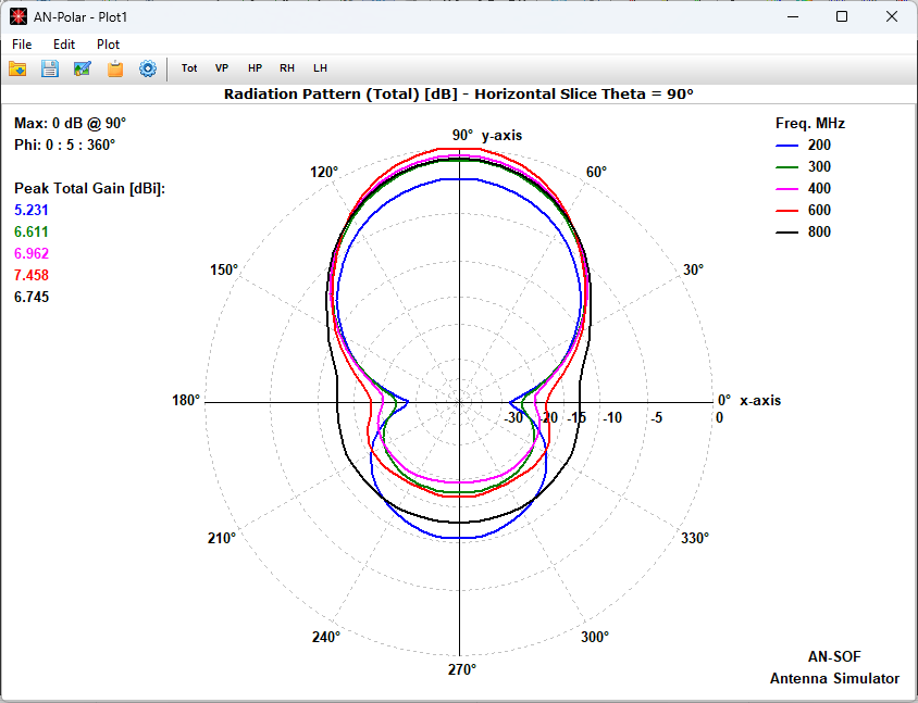
2. In the configuration window (Fig. 6), select the cut orientation (Fixed $\theta$ or Fixed $\phi$).
3. Choose up to five active frequencies from your pre-calculated sweep.

🗒️ Example (Fig. 6): A fixed angle of $\theta = 90^\circ$ is selected. Five slices are enabled to compare the antenna’s azimuthal performance at: $200\text{ MHz}$ (Slice 1), $300\text{ MHz}$ (Slice 2), $400\text{ MHz}$ (Slice 3), $600\text{ MHz}$ (Slice 4), and $800\text{ MHz}$ (Slice 5).

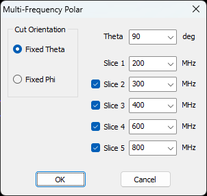
Figure 7 shows the resulting five-slice plot within AN-Polar. A color-coded legend in the upper-right corner identifies each frequency, and the corresponding peak total gain values are tabulated on the left for quick reference.

5. Comparing Different Antennas (Export and Import)

To compare different antenna designs or geometric iterations in a single polar diagram, you can export and import pattern data using AN-SOF’s proprietary .plr format.

💡 Tip: You do not need to load or run an active simulation project to view saved plots. To open and inspect previously saved .plr files, you can launch the AN-Polar application independently from the AN-SOF main interface by navigating to Tools > Polar Chart Application…

5.1. Exporting a Polar Slice

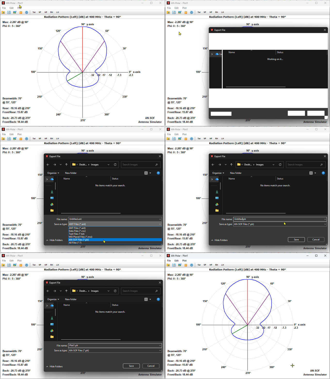
1. Open the source radiation pattern in AN-Polar.
2. Navigate to File > Export…
3. Select the file filter AN-SOF File (*.plr).
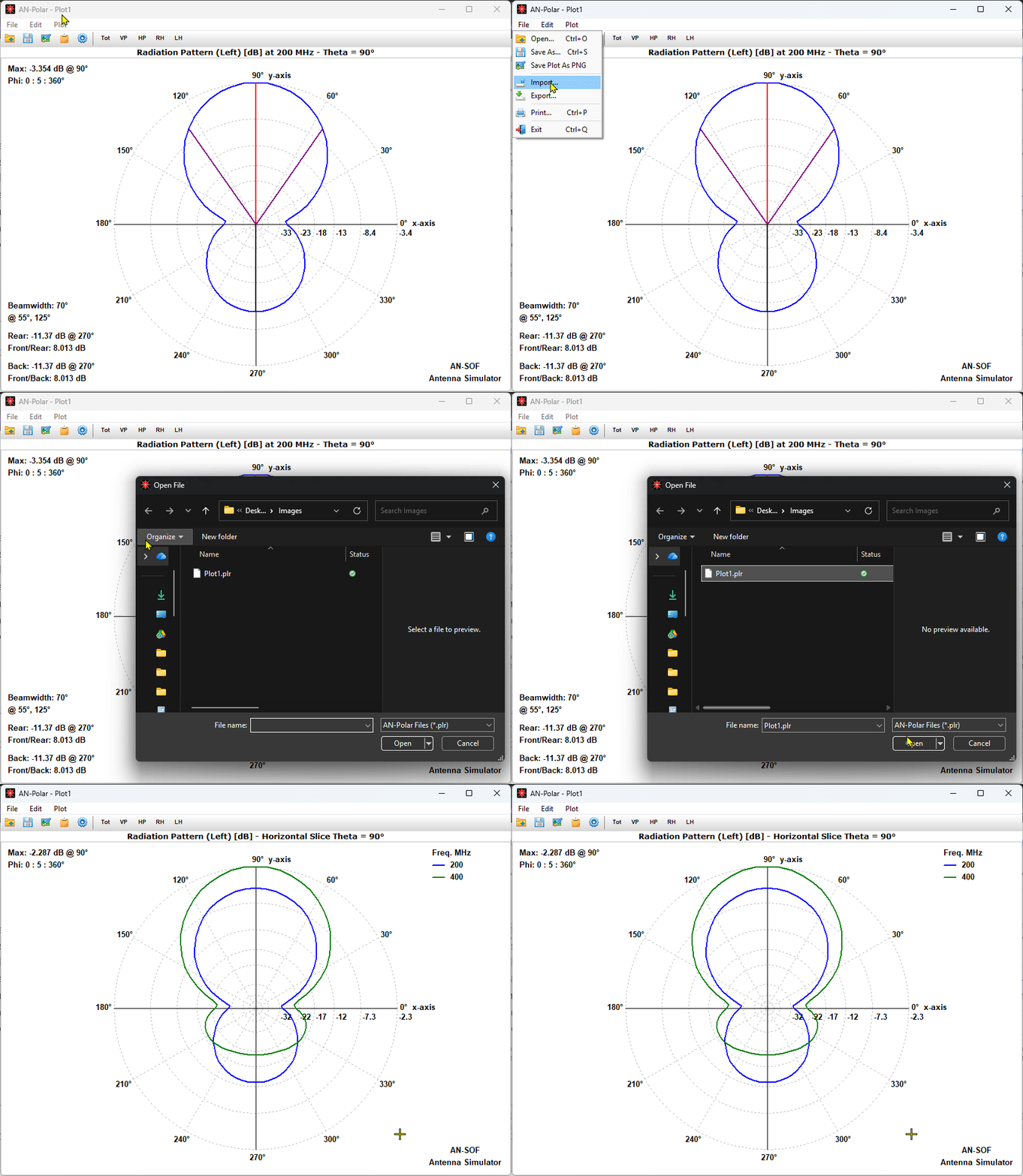
4. Enter a name (e.g., Plot1.plr, as in Fig. 8) and click Save.

Note: If the active plot consists of multiple slices, only Slice 1 will be exported to the .plr file.

5.2. Importing Slices to a Composite Plot

1. Open a single-slice polar plot of your baseline antenna by selecting: Results > Far-Field Angular Plot > Single Slice Polar…
2. In the AN-Polar main menu, navigate to File > Import…
3. Select the previously exported file (e.g., Plot1.plr, as in Fig. 9).
4. Repeat this process to import up to four external slices. This allows you to display a total of five distinct antenna patterns in a single polar plot.
5. To save this composite plot for subsequent review, select File > Save As… to create a master .plr file.

5.3. Editing Legends and Aligning Orientations

When combining multiple antenna patterns, it is often necessary to clean up the plot legend and account for different physical orientations:

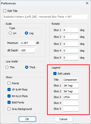
• Legend Customization: Go to Edit > Preferences… (or click the Gear icon on the toolbar) to open the Preferences window (Fig. 10). Here, you can customize the main legend title and edit individual labels for Slices 1 to 5 to clearly identify each antenna model.
• Coordinate Rotation: If the imported antennas were modeled with different physical orientations, you can specify an individual rotation angle (in degrees) for each slice within the same Preferences window to align the patterns for a consistent comparison.

6. Saving and Exporting in Alternative Formats

While the .plr format is ideal for saving complete polar plot sessions (opened via File > Open), you may need to share raw data with external applications.

Navigate to File > Export… and select one of the following formats:

• .ant (Radio Mobile software format)
• .msi (MSI Planet format for telecommunication planning)
• .txt / .csv (Raw tabulated text data containing angles and amplitudes)

Note: When exporting a multi-slice or multi-frequency plot to these external formats, only the active Slice 1 data will be exported.

7. Conclusions

The multi-slice and multi-frequency capabilities of the AN-Polar application provide a highly efficient, visual method for evaluating antenna performance. By allowing up to five distinct slices to be plotted simultaneously, the software eliminates the need for tedious manual data correlation. The slices to be plotted simultaneously can come from different angular cuts, frequency steps, or separate antenna files.

When conducting these analyses, maintaining proper dynamic range through scale customization (linear vs. ARRL logarithmic) and utilizing polarization decomposition tools ensures that both primary radiation characteristics and secondary sidelobe effects are represented with high scientific accuracy.

8. See Also:

• Front-to-Rear and Front-to-Back Ratios: Applying Key Antenna Directivity Metrics

• Exporting Radiation Patterns to Radio Mobile: A Step-by-Step Guide

• Exporting Radiation Patterns to MSI Planet Format: A Step-by-Step Guide

Technical Keywords: antenna far-field comparison, multi-slice polar plot, multi-frequency polar plot, radiation pattern overlay, AN-SOF, AN-Polar, PLR format, polarization decomposition, horizontal cut, vertical cut, ARRL scale, LPDA simulation, peak total gain, antenna directivity, vertical polarization, horizontal polarization, circular polarization, MSI Planet format, Radio Mobile antenna, electromagnetic pattern visualization, antenna simulation data export.

---