Introducing AN-SOF 11: Precision Modeling and Next-Gen Electromagnetic Simulation

Created OnJuly 8, 2026

Updated OnJuly 9, 2026

By:Tony Golden

We are thrilled to announce the release of AN-SOF Antenna Simulator Version 11. This landmark update introduces major advancements in our core electromagnetic solver, significantly expands the modeling CAD toolbox, and delivers highly requested visualization tools for RF engineers, academic researchers, and antenna design enthusiasts.

By implementing Richmond’s method for coated wires, introducing automatic bandwidth calculation, and adding advanced geometry manipulation tools like mouse-driven wire joining and smart wire-checking routines, AN-SOF 11 empowers you to model closer to real-world scenarios with unprecedented speed and accuracy.

1. Electromagnetic Solver & Material Modeling

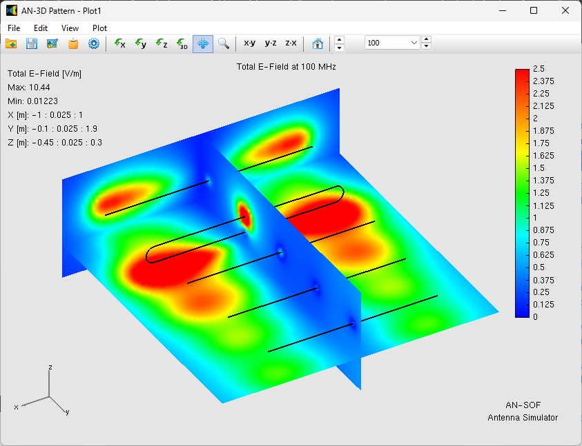
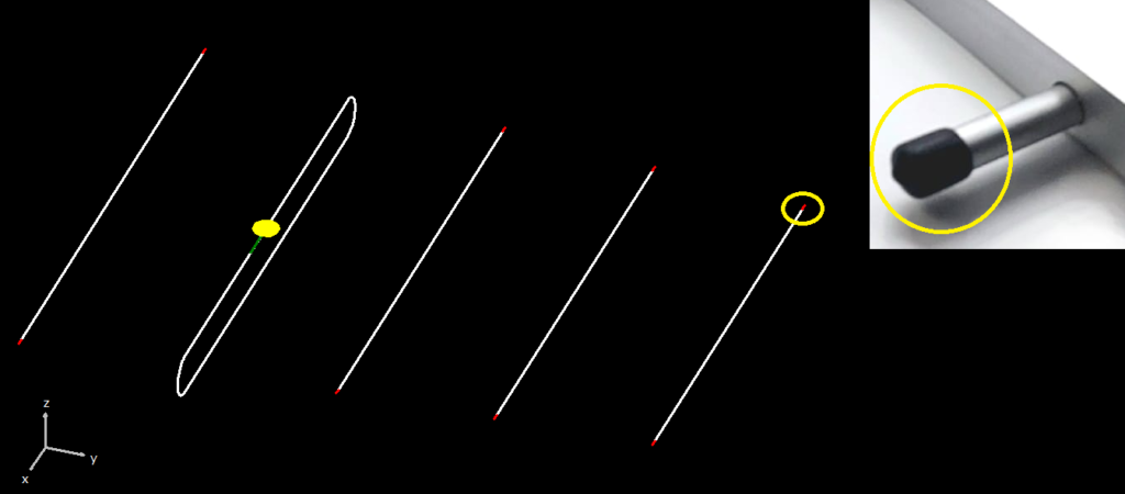
Richmond’s Method for Insulated Wires: We have fully implemented Richmond’s method for modeling magneto-dielectric coated wires. Known as the most mathematically rigorous approach for coated conductors, this implementation makes AN-SOF the most accurate tool on the market for simulating insulated wires (Fig. 1).

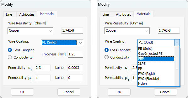
Comprehensive Preset Materials Database: A dedicated materials database has been added to the Materials tab. You can now select from pre-configured lists of dielectrics, magneto-dielectrics, and meta-materials with pre-defined permittivity (dielectric constant $\varepsilon_{r}$), magnetic permeability ($\mu_{r}$), and electric/magnetic loss tangents ($\tan \delta$) (Fig. 2).

Enhanced Skin-Effect Accuracy: The skin-effect calculation engine has been optimized for superior accuracy. It now delivers highly precise loss modeling for standard circular wires as well as non-circular cross-sections, including rectangular conductive strips and square antenna booms.

**Fig. 1:** Richmond’s method precisely models the effect of plastic end caps used to insulate and protect the tips of antenna elements. These caps increase the elements’ electrical length, thereby lowering the resonant frequency.

**Fig. 2:** The updated **Materials** tab, where users can configure wire resistivity (to account for skin-effect losses) and apply custom magneto-dielectric coatings.

2. CAD, Geometry & Modeling Workflow

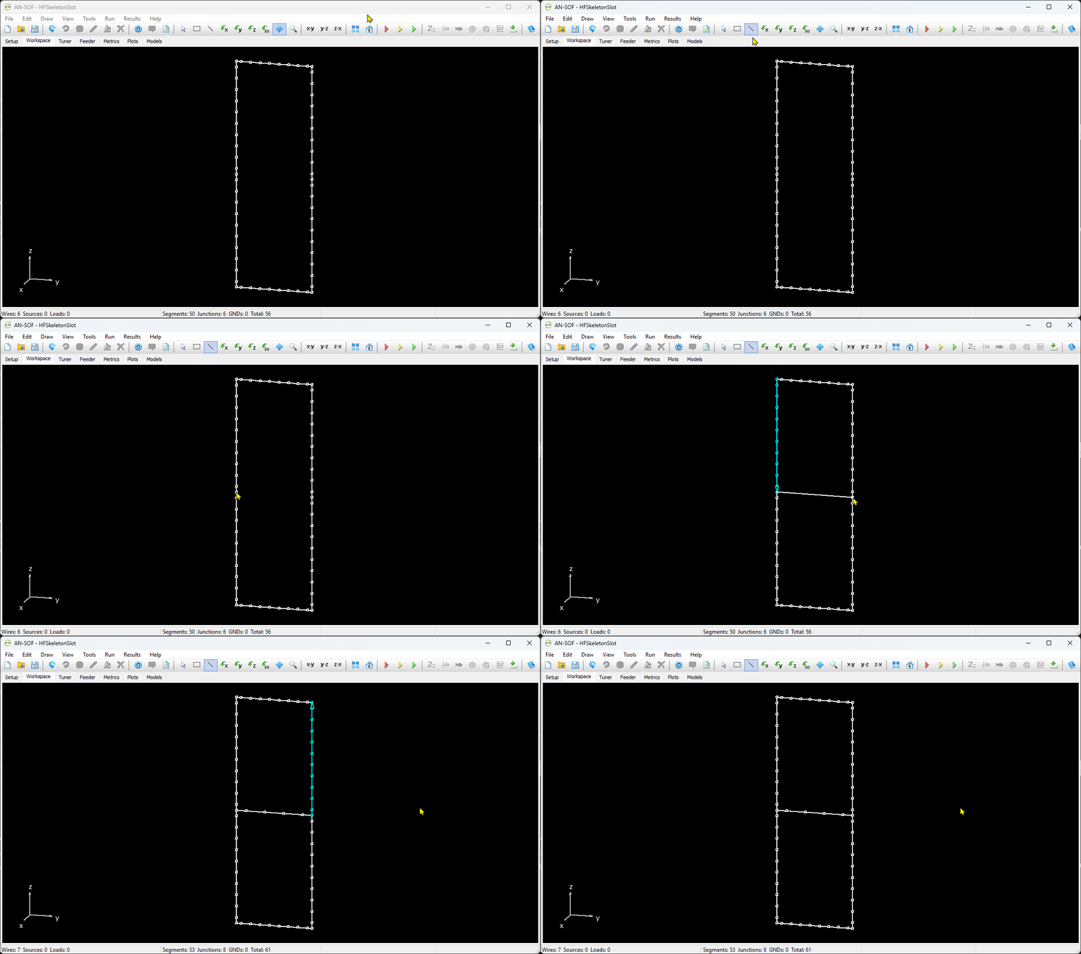
Interactive “Join Wires” Tool: A new “Join Wires” button has been added directly to the main toolbar. You can now easily connect wire start/end points visually by dragging a line between endpoints in the 3D workspace (Fig. 3).

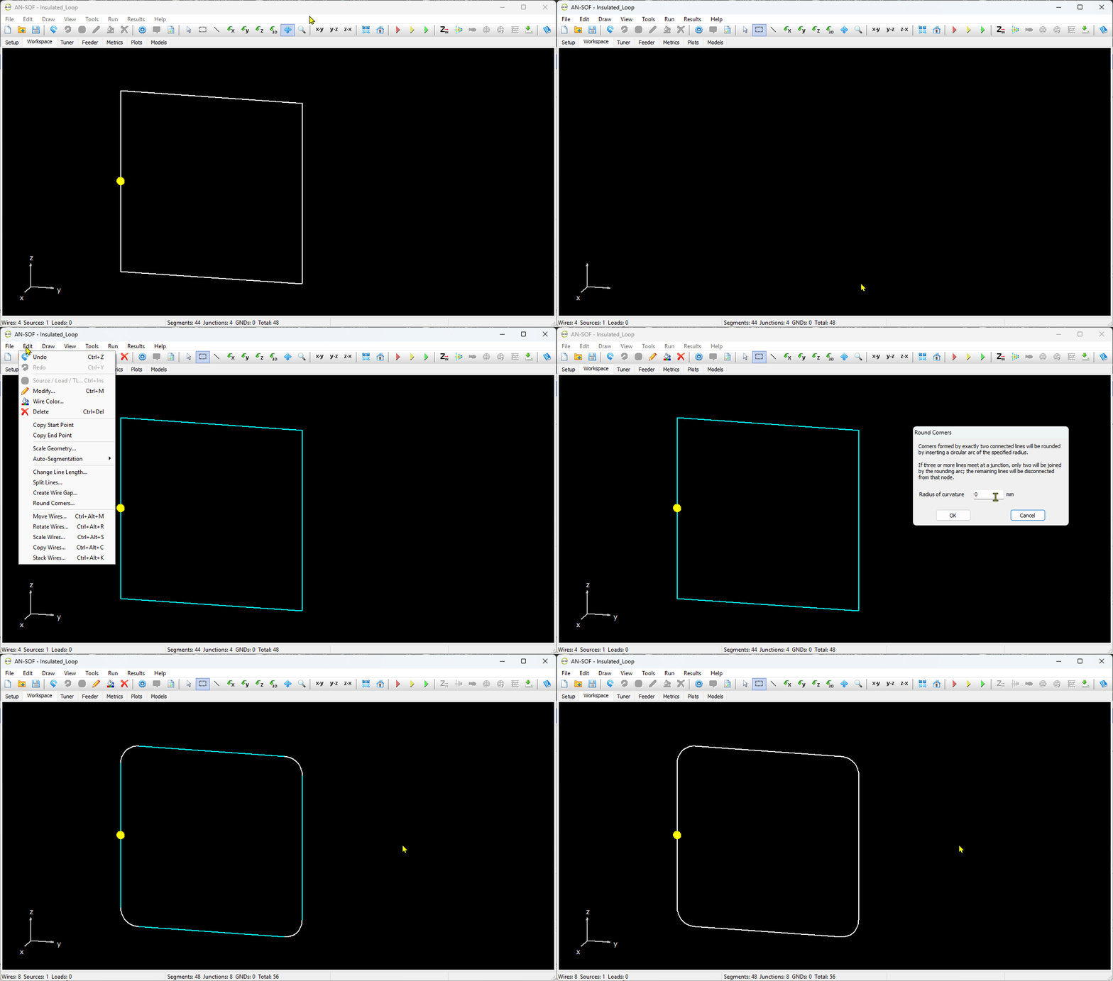
**Fig. 3:** Visually connecting wire endpoints by dragging a line with the mouse directly within the 3D workspace.

“Round Corners” Junction Command: Easily round sharp corners (where two wires meet at an acute angle) by selecting them and specifying a radius of curvature. This feature leverages the Conformal Method of Moments (CMoM) capability to accurately model physical wire bends as they exist in real-world construction (Fig. 4).

**Fig. 4:** Rounding the corners of a square loop antenna. Because physical insulated wires cannot be bent at perfectly sharp, acute angles, this feature is essential for modeling the actual radius of curvature of the bend.

Spreadsheet-Style Tabular Input Upgrades: For users accustomed to NEC-style spreadsheet workflows, the Tabular Input (Ctrl + T) has been heavily optimized:
- Added options to shift coordinates and adjust lengths of wires.
- Integrated wire insulation loss tangent ($\tan \delta$) inputs directly into the tables.
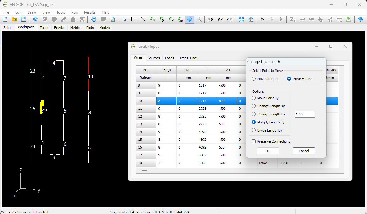
- Added a “Preserve Connections” option when editing lengths to ensure adjacent structures stretch or compress dynamically without disconnecting (Fig. 5).

**Fig. 5:** Modifying the length of a selected wire directly within the optimized, spreadsheet-style **Tabular Input** window.

Dynamic Command Transformations: The “Preserve Connections” mechanism has also been integrated into the standard Move, Rotate, and Scale Wires edit operations, preventing broken geometry during complex transformations.

New Edit Menu Operations:

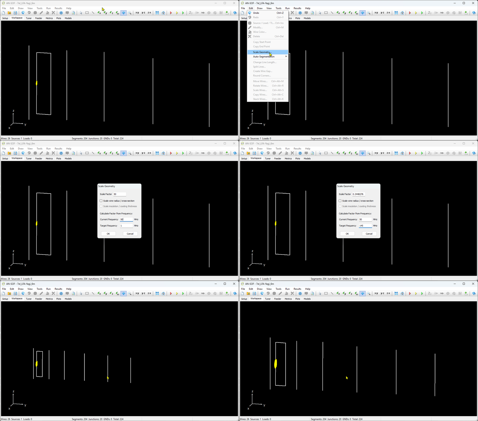
Scale Geometry: Rescale your entire structural model uniformly. The scaling factor can be entered manually or calculated dynamically by entering a current frequency and a target design frequency (Fig. 6).

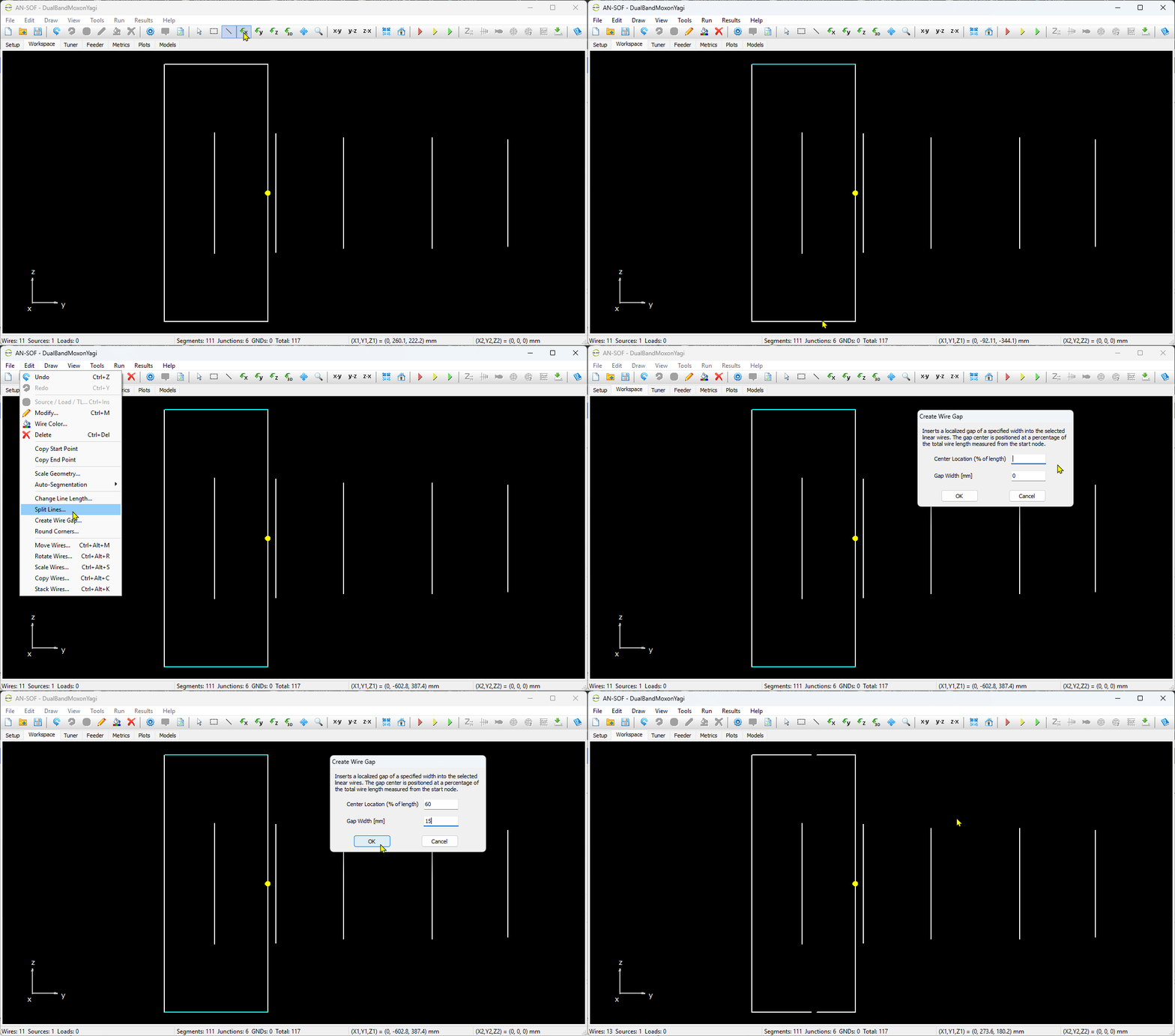
**Fig. 6:** Uniformly scaling the entire antenna geometry by entering a current design frequency and a target operating frequency.

Create Wire Gap: Quickly slice a precise gap into a wire (Fig. 7). This simplifies the construction of antennas with wire gaps like Moxons, and provides clean attachment points for bridging wires in order to model feed-points, where a source is connected to the bridging wire, or to precisely position load impedances by connecting a load to the bridging wire.

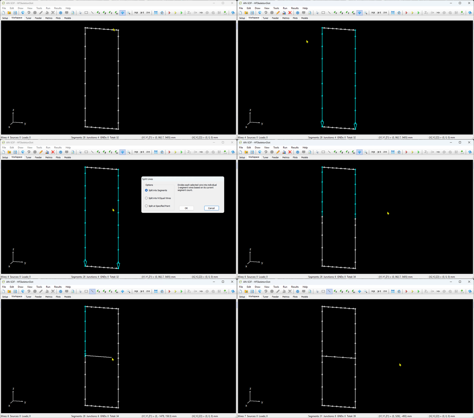
**Fig. 7:** Slicing a precise wire gap into a square loop to construct a Moxon antenna element, designed here as part of a directive Moxon-Yagi array.

Split Wires: Subdivide selected wires into a specified number of portions, by their number of segments, or split a single wire in two at an exact coordinate (Fig. 8).

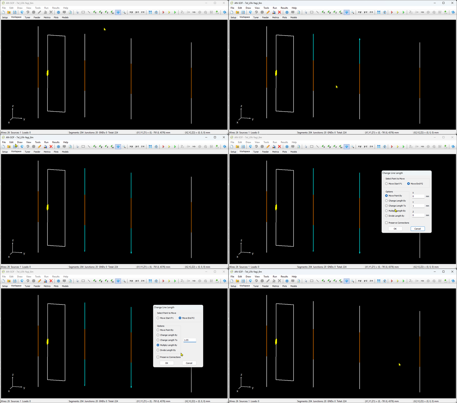
**Fig. 8:** Subdividing the wires of a rectangular loop and visually joining them in the workspace to construct a skeleton slot antenna.

Change Line Length: Rapidly alter selected wire lengths with full “Preserve Connections” support (Fig. 9).

**Fig. 9:** Selecting specific wires via point-and-click in the workspace to dynamically adjust their physical lengths.

Model Validation & Verification Routines: The three intelligent wire checking commands in the Tools menu have been optimized to eliminate hidden modeling errors before running calculations:
- Delete Duplicate Wires: Improved algorithmic checks to eliminate redundant wires while preventing false positives on closely spaced parallel components.
- Check Wire Spacing: Instantly identifies overlapping or intersecting wires that violate spacing constraints.
- Check Individual Wires: Flags wires that accidentally cross, touch, or fall below the ground plane boundary.

Array Building Enhancements: The Copy Wires and Stack Wires tools now feature optional checkmarks to Preserve Sources and Preserve Loads, exponentially reducing the manual setup time required to build complex phased arrays.

Smart AWG Entry Support: You can now enter wire radii directly as an AWG size (e.g., #14). Upon hitting ENTER, the software automatically calculates and converts the gauge into the numeric value of your active unit system (inches, millimeters, etc.) (Fig. 10).

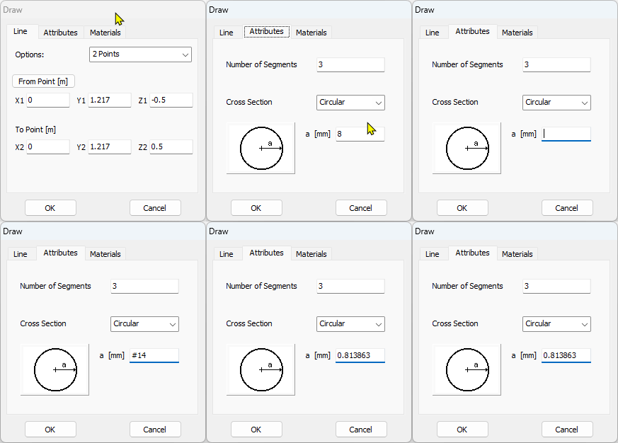
**Fig. 10:** Enter `#` followed by the AWG wire gauge (e.g., `#14`) and press `ENTER` to automatically calculate and display the corresponding wire radius in the active unit system.

Additional Modeling Utilities:

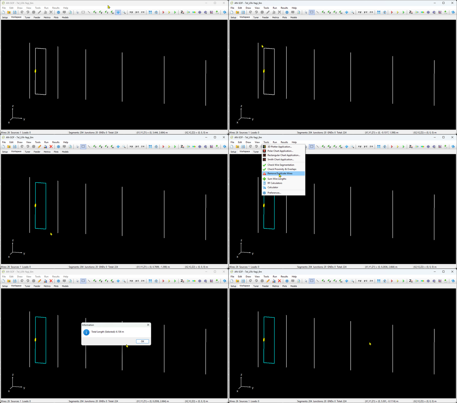
Sum Wire Lengths: Displays the aggregate length of selected wires or the entire structure via the Tools menu (Fig. 11).

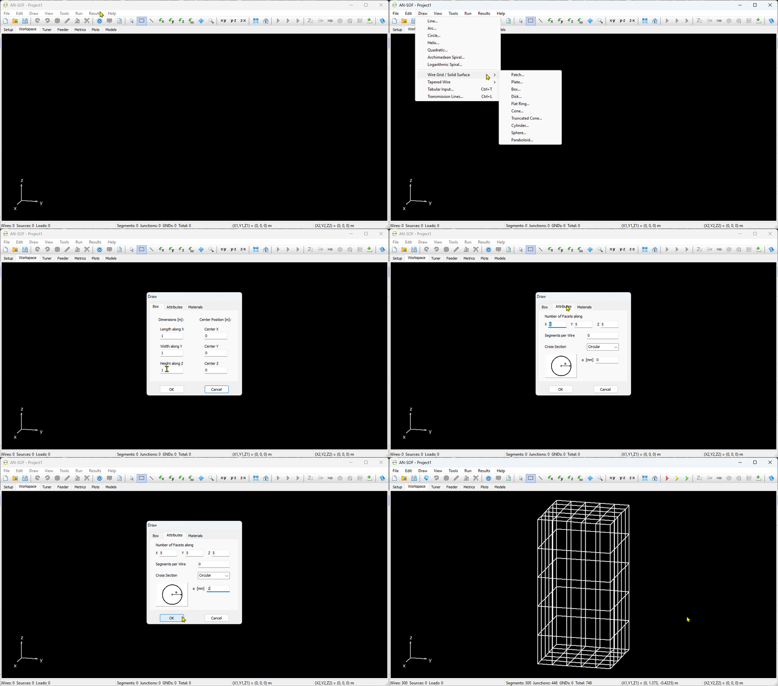
**Fig. 11:** Calculating the cumulative physical length of a group of selected wires using the **Tools > Sum Wire Lengths** command.

Box Wire Grid/Solid Surface: Quickly add box-shaped structures to wire grids and solid surface models (Fig. 12).

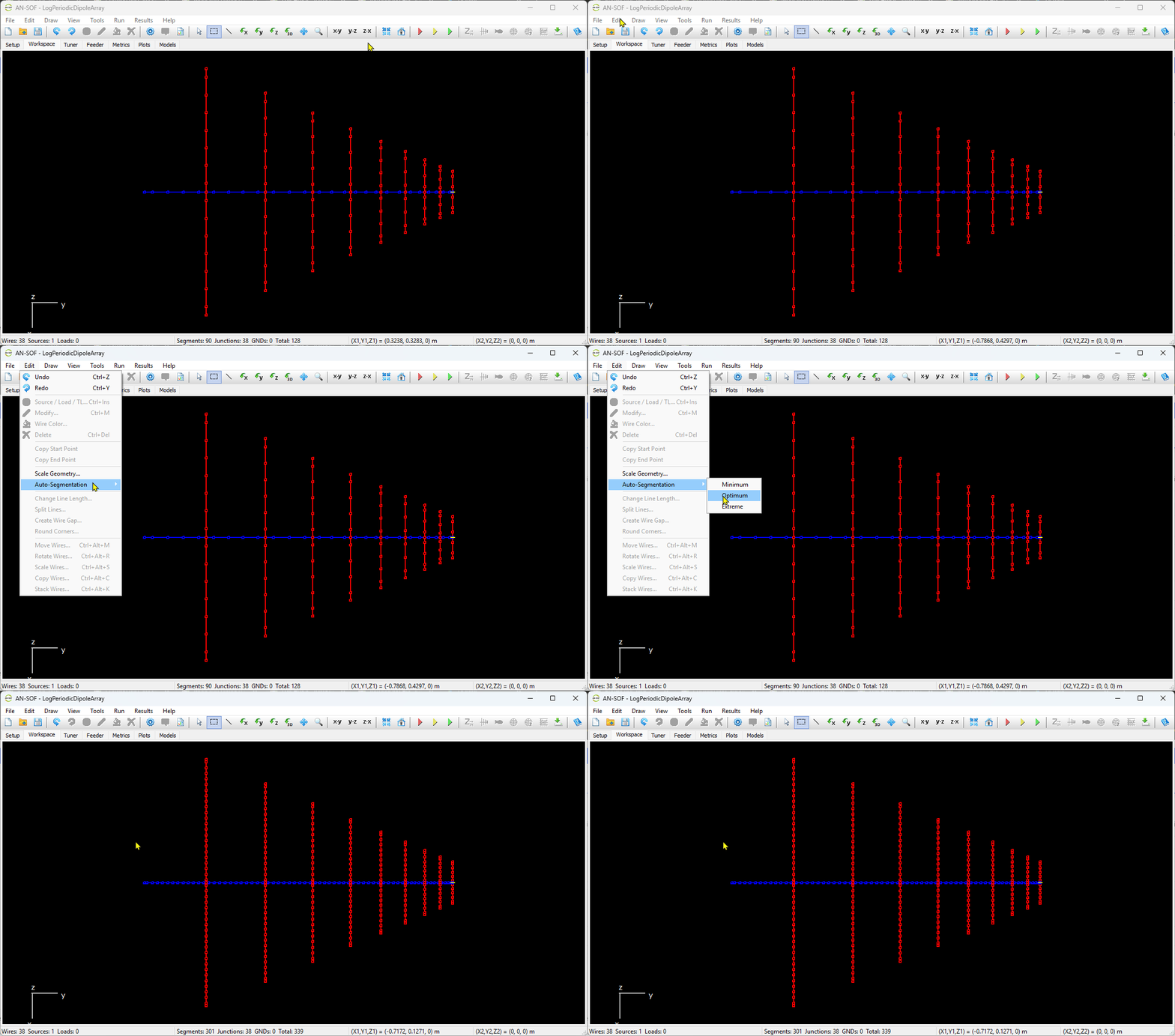
**Fig. 12:** Instantly adding a pre-configured box modeled as a wire grid structure.

Auto-Segmentation Options: Preset segmentation rules have been added to the Edit menu to enforce standard densities effortlessly: Minimum ($10\text{ segs}/\lambda$), Optimum ($20\text{ segs}/\lambda$), and Extreme ($50\text{ segs}/\lambda$) (Fig. 13).

**Fig. 13:** Choosing the **Optimum** auto-segmentation option in the **Edit** menu to automatically discretize a Log-Periodic Dipole Array (LPDA) into 20 segments per wavelength.

3. Analysis, Calculations & Metrics

Automatic Bandwidth Calculator: Incorporated directly into the Plots tab. When analyzing your $\text{VSWR}/S_{11}$ plot, the calculator automatically displays the absolute bandwidth, fractional bandwidth ($\%$), minimum and maximum operational frequencies, and center frequency (defined as the minimum VSWR point). It also flags the true first physical resonance point where the input reactance $X_{\text{in}} = 0$ (Fig. 14).

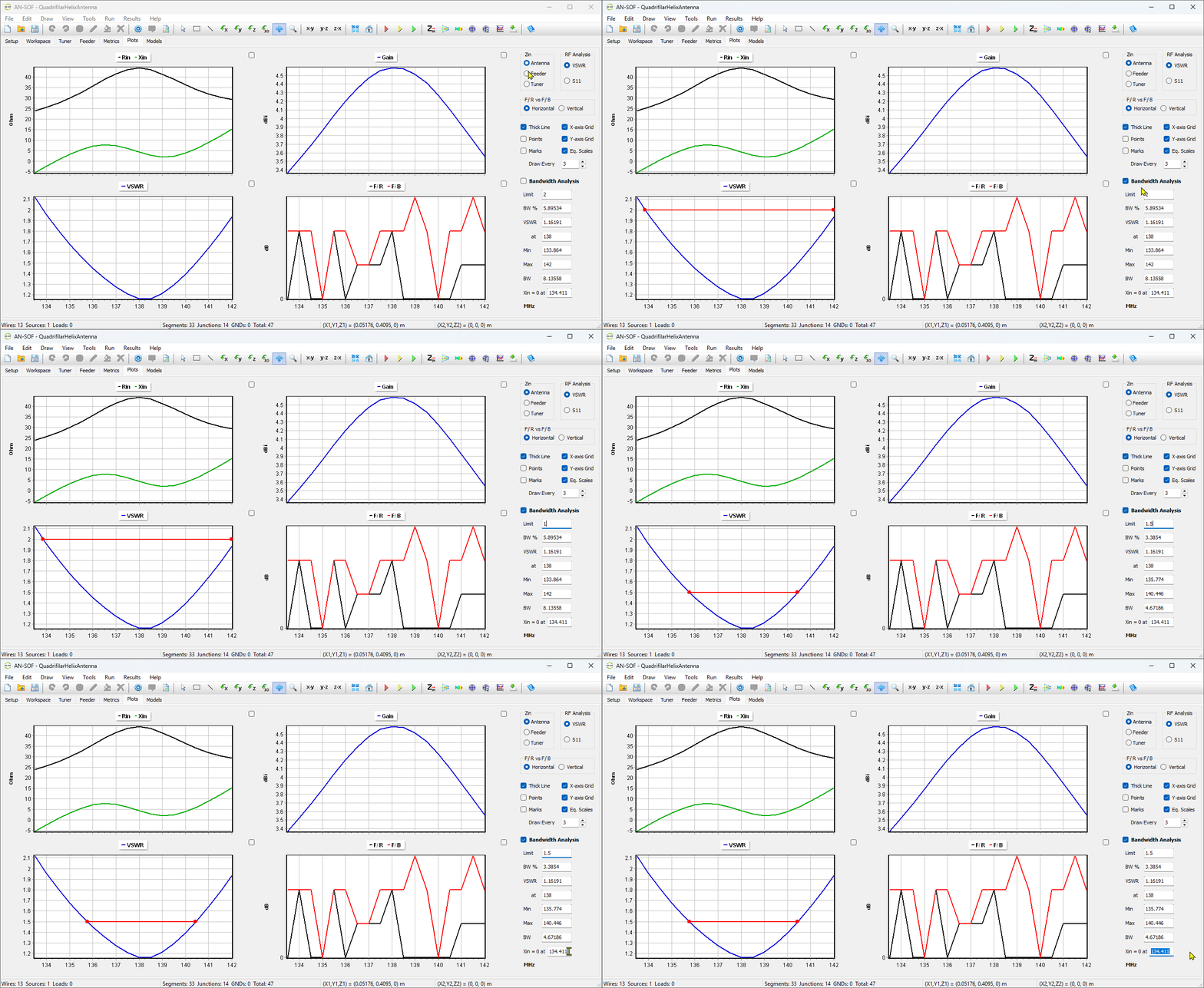
**Fig. 14:** The integrated Bandwidth Calculator in the **Plots** tab. Define a target VSWR threshold (typically 1.5 or 2.0) and press `ENTER` to instantly calculate absolute bandwidth, fractional bandwidth, and associated frequencies.

Multi-Plane Orthogonal Near-Field Assessment: For Electromagnetic Field (EMF) safety compliance and exclusion-zone modeling, you can now define and calculate near fields ($E$, $H$, and $S$) simultaneously across three orthogonal planes, eliminating the need to set up, calculate, and export one plane at a time (Fig. 15).

**Fig. 15:** Near-zone electric field (E-field) distribution surrounding a 5-element Yagi-Uda antenna, calculated simultaneously across three orthogonal planes.

Interactive Metrics Panel (formerly Results):

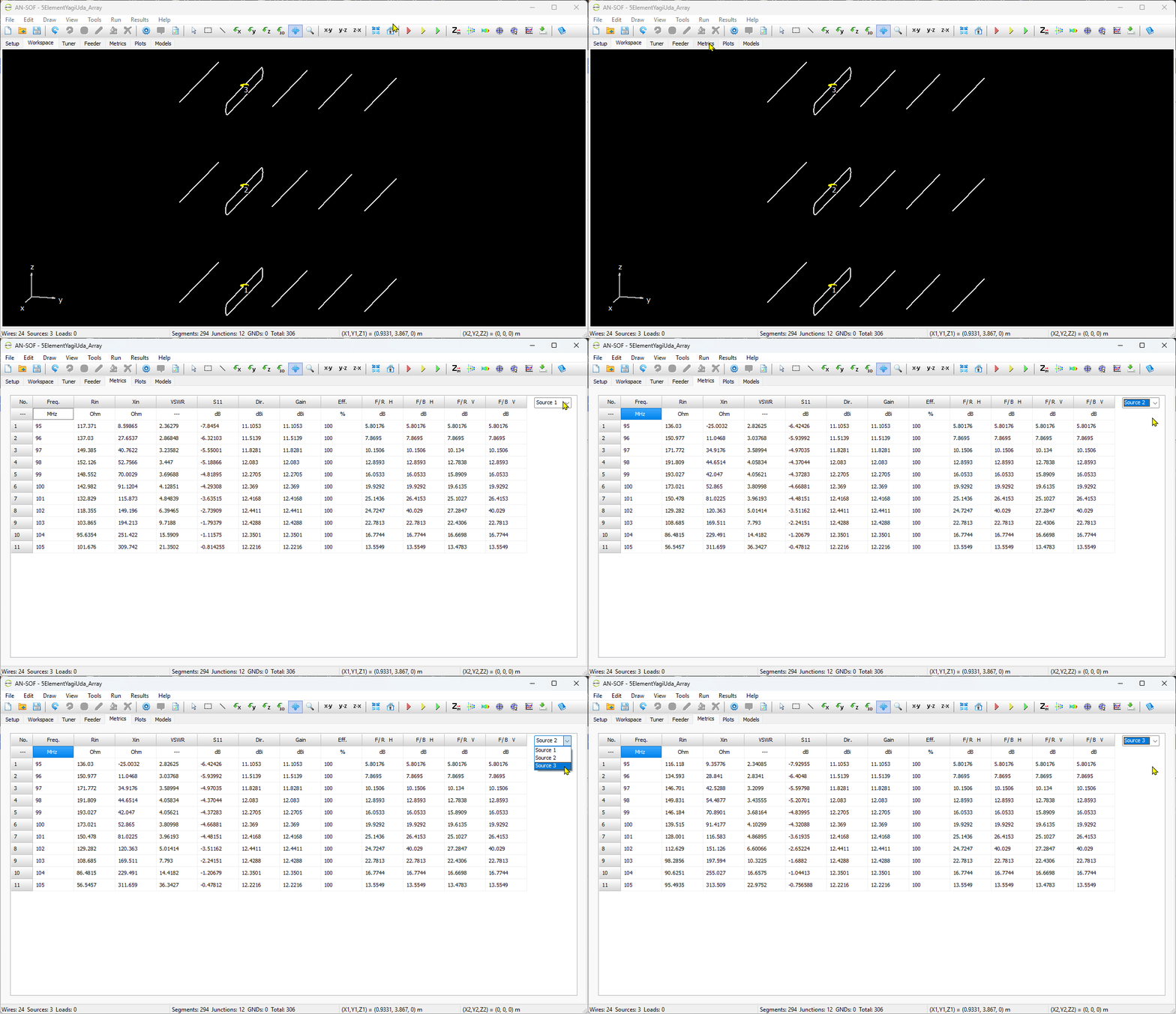
The Metrics tab now contains a dynamic source list. For multi-source configurations (such as phased arrays), selecting a source from the list instantly updates all corresponding feedport impedance and related metrics across the Plots and Metrics views (Fig. 16).

The active source numbering layout is projected directly into the 3D workspace alongside the antenna geometry for instant visual reference.

Port metrics automatically cascade to the Input Impedance Table toolbar command.

**Fig. 16:** For multi-source configurations (such as phased arrays), selecting an active port from the source list dynamically updates all relevant feedpoint metrics across both the **Metrics** and **Plots** views.

4. GUI, Plotting & Visualization

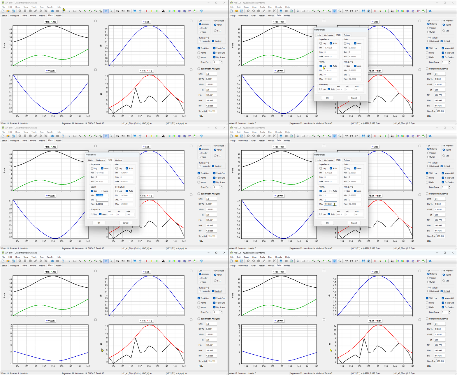
Complete Axes and Scales Control: Tailor your data representation. New preferences in AN-SOF and AN-XY Chart allow you to customize minimums, maximums, linear/logarithmic scales, step increments, and toggles for global auto-scaling (Fig. 17).

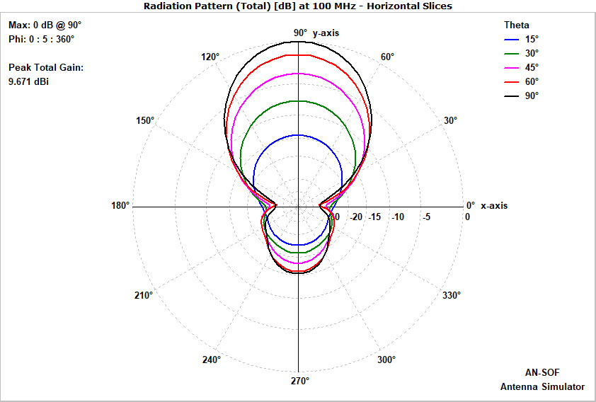
**Fig. 17:** The updated **Plots** preferences tab in the **Preferences** window, providing complete control over axis limits, linear/logarithmic scaling, and step increments.

Advanced Multi-Slice AN-Polar Display: The AN-Polar app now supports plotting up to 5 slices simultaneously across varying azimuth/zenith angles or frequencies (Fig. 18).

**Fig. 18:** The Multi-Slice Polar feature within the **Results > Far-Field Angular Plot** menu enables simultaneous plotting of up to 5 radiation pattern slices.

External Pattern Import & Overlays: You can now import polar patterns from external projects to compare antennas, apply slice rotation, and edit legends (Fig. 19).

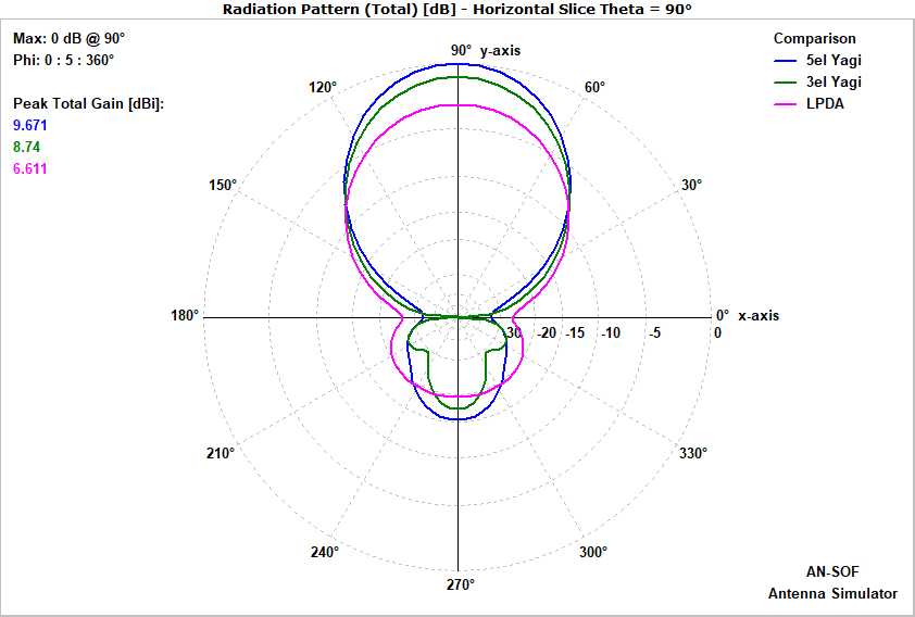
**Fig. 19:** Overlaying up to 5 imported radiation patterns from external design projects onto a single polar chart is now possible for direct performance comparison.

Peak Total Gain Overlay: When showing a normalized radiation pattern (scaled $0$ to $1$, or $-100\text{ dB}$ to $0\text{ dB}$) in the AN-Polar app, the Peak Total Gain is printed directly next to the polar plot, preventing the need to toggle back and forth between normalized and absolute gain plots.

System Print Support: A native Print option is now available across all plotting applications and the primary AN-SOF application, allowing you to route high-resolution graphs, charts, and geometry screenshots directly to your physical or PDF printer.

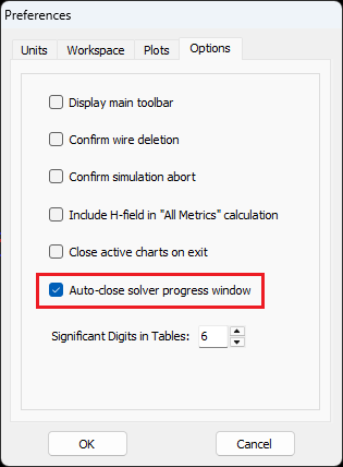
Auto-Close Progress Dialog: A new toggle in Preferences > Options allows the solver progress window to auto-close immediately following a successful simulation run, smoothing out high-iteration modeling sweeps (Fig. 20).

**Fig. 20:** Enabling the optional auto-close toggle for the solver progress window within the program **Preferences** allows users to streamline highly iterative sweep workflows.

5. File Formats, Import & Export Integration

Enhanced NEC Compatibility: The insulation loss tangent ($\tan \delta$) of coated wires is now successfully mapped, read, and preserved when importing or exporting standard .nec files.

Advanced Scripting Export Templates: When exporting your wire structures to Scilab (.sce files) or Octave/MATLAB (.m files) to run external optimization routines, wire insulation loss tangents are fully integrated into the auto-generated scripts.

Looking Ahead

We are incredibly excited for you to experience the streamlined workflow, expanded material databases, and deeper visual plotting capabilities of AN-SOF 11. This major update represents our commitment to continuously improving accuracy and usability based directly on your invaluable feedback. We cannot wait to see what amazing designs and discoveries you bring to life using this new toolkit.

As always, thank you for being a vital part of our global community.

Warm regards,

Tony Golden

About the Author

Tony Golden

RF ENGINEER & PHYSICS PH.D. With 25+ years in Computational Electromagnetics, I’m a passionate researcher focused on antenna modeling and design. As Founder of Golden Engineering LLC, I develop accessible, high-performance simulation tools that help RF engineers optimize their designs, educators teach complex concepts, and hobbyists bring antenna projects to life.