Evolving Better Antennas: A Genetic Algorithm Optimizer Using AN-SOF and Scilab

Learn to optimize antennas with genetic algorithms using AN-SOF and Scilab. Includes ready-to-use scripts for population evolution and cost functions targeting gain, VSWR, and front-to-back ratio in a 3-element Yagi-Uda design.

Harnessing Genetic Algorithms for Antenna Design Optimization

Genetic Algorithms (GAs) offer a powerful approach to antenna optimization by emulating biological evolution. Unlike traditional methods that iteratively refine a single design, GAs maintain a population of potential solutions that gradually evolve toward optimal performance. This population-based strategy makes GAs particularly effective for complex antenna systems where the relationship between design parameters and performance metrics is highly nonlinear or involves multiple competing objectives.

At the core of a GA implementation are several key concepts. The process begins by encoding antenna parameters—such as element lengths, spacings, or feed positions—into digital chromosomes that represent individual designs. These designs then undergo repeated cycles of evaluation, selection, and modification. During each generation, the algorithm assesses design fitness using a cost function that quantifies performance metrics like gain, bandwidth, or impedance matching. The most successful designs are selected to produce offspring through crossover operations, while random mutations introduce valuable diversity into the population.

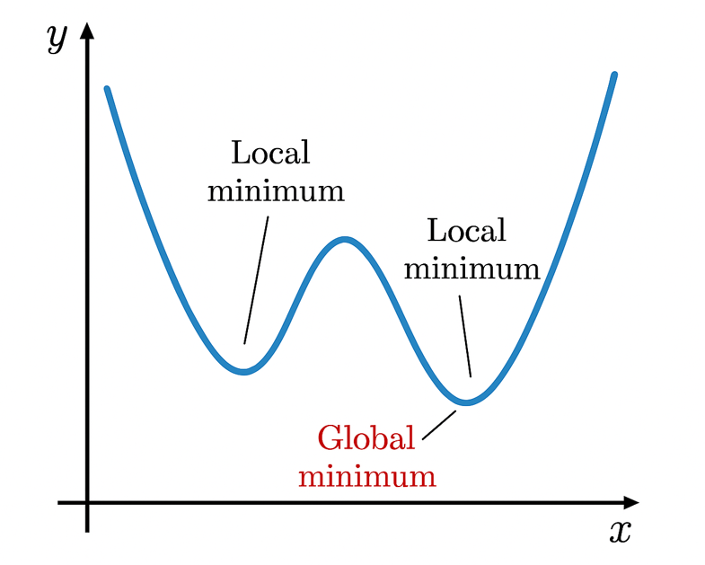
The advantages of GAs become particularly apparent when optimizing challenging antenna configurations. Their ability to explore multiple design trajectories simultaneously helps avoid convergence to suboptimal local minima (Fig. 1), a common limitation of gradient-based methods. Furthermore, GAs can naturally handle multi-objective optimization problems, such as simultaneously maximizing gain while minimizing sidelobe levels across multiple frequency bands. This flexibility extends to various antenna types, from simple dipoles to complex fractal arrays and metasurface designs.

This article demonstrates a GA optimization workflow using Scilab’s built-in genetic algorithm functions coupled with AN-SOF Engine for full-wave EM analysis. While the core script operation – including NEC file generation, simulation execution, and result processing – remains identical to our previous Nelder-Mead implementation, the key difference lies in the optimization engine. Here, we replace the Nelder-Mead method with Scilab’s optim_ga() function, enabling population-based exploration of the design space and improved handling of multi-modal optimization problems.

Summary: Genetic Algorithm Workflow

How GAs Work:

1. Population-Based Search:
   • Starts with multiple random designs (“chromosomes”) encoding antenna parameters (e.g., lengths, spacings).
   • Example: A 3-element Yagi-Uda chromosome might be [d₁ = 0.2λ, d₂ = 0.15λ, L₁ = 0.45λ], where d₁ and d₂ are element spacings and L₁ is the driven element length.
2. Fitness Evaluation:
   • Each design is scored by a cost function (e.g., weighted sum of VSWR, gain, front-to-back ratio).
3. Selection & Reproduction:
   • Top-performing designs “mate” to create offspring with combined traits.
   • Random mutations maintain diversity.
4. Iterative Refinement:
   • Over generations, the population evolves toward optimal solutions.

Advantages for Antenna Design:

• Global Optimization: Avoids local minima traps common in gradient-based methods.
• Multi-Objective Handling: Simultaneously optimizes gain, bandwidth, and matching via fitness weighting.
• Geometry Flexibility: Optimizes complex structures (fractals, metasurfaces) without derivative calculations.

Script Functions and Cost Function Implementation

The Role of the Cost Function

In Genetic Algorithms, the cost function acts as the “fitness test” that evaluates each antenna design in the population. It quantifies how close a design comes to meeting your targets (e.g., desired gain, VSWR, or front-to-back ratio). The GA uses these cost values to:

• Select the best-performing designs for reproduction
• Drive the population toward optimal solutions over generations
• Balance trade-offs between competing objectives

Required Scripts

1. NECcommands.sce
   • Must be executed first to load AN-SOF-compatible NEC functions into Scilab.
   • Contains all supported GW, EX, FR, etc. commands for antenna modeling.
2. GAoptimizer.sce
   • The main Genetic Algorithm script, run after NECcommands.sce.
   • Implements population generation, selection, and the optimization loop.

Download Resources:

(Includes both NECcommands.sce and GAOptimizer.sce files)

Core Functions (Same as Nelder-Mead)

1. modify_nec_file(filename, params)
   Updates the .nec file with current design parameters (e.g., spacings, lengths).
2. read_antenna_results(filename)
   Extracts VSWR, gain (G), and horizontal front-to-back ratio (FBH) from AN-SOF’s output CSV.
3. antenna_cost(params)
   • Calls the above functions and the AN-SOF Engine to simulate and evaluate a design.
   • Computes the weighted cost (below) to guide the GA.

Cost Function Formula

cost = (VSWR_W · ΔVSWR + G_W · ΔG + FBH_W · ΔFBH) / (VSWR_W + G_W + FBH_W)

where:

• ΔVSWR = |VSWR − VSWR₀| / VSWR₀
• ΔG = |G − G₀| / G₀
• ΔFBH = |FBH − FBH₀| / FBH₀

The goal is to achieve specific target values for three key performance metrics:

• VSWR₀ (voltage standing wave ratio)
• G₀ (gain)
• FBH₀ (horizontal front-to-back ratio)

Why This Works:

• Normalized Errors: % deviations ensure fair weighting across parameters.
• Customizable Priorities: Adjust weights (VSWR_W, G_W, FBH_W) to emphasize critical specs.

AN-SOF Engine Integration

The antenna_cost function automatically executes the AN-SOF Engine—our high-performance Conformal Method of Moments (CMoM) simulator—to evaluate each antenna design. When called, it:

1. Generates a .nec file with the current parameters
2. Runs a full-wave EM simulation via AN-SOF’s solver
3. Extracts key results (VSWR, gain patterns, impedance)

This seamless integration enables accurate evaluation of each design’s electromagnetic performance before cost calculation. For installation and licensing details, visit the AN-SOF Engine User Guide.

For full implementation details, see:

• Nelder-Mead Optimization for Antenna Design Using the AN-SOF Engine and Scilab

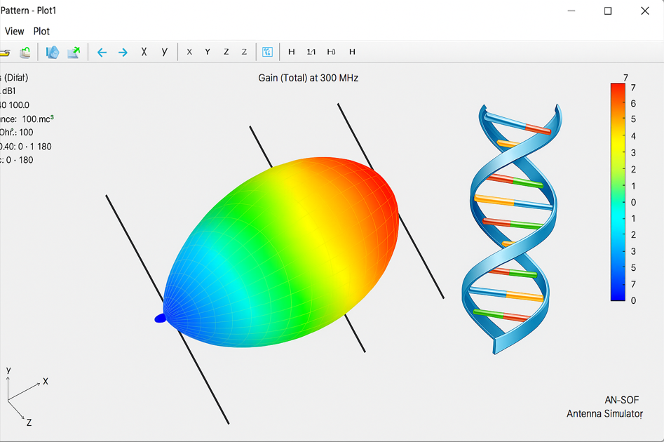
Yagi-Uda Geometry and Optimization Parameters

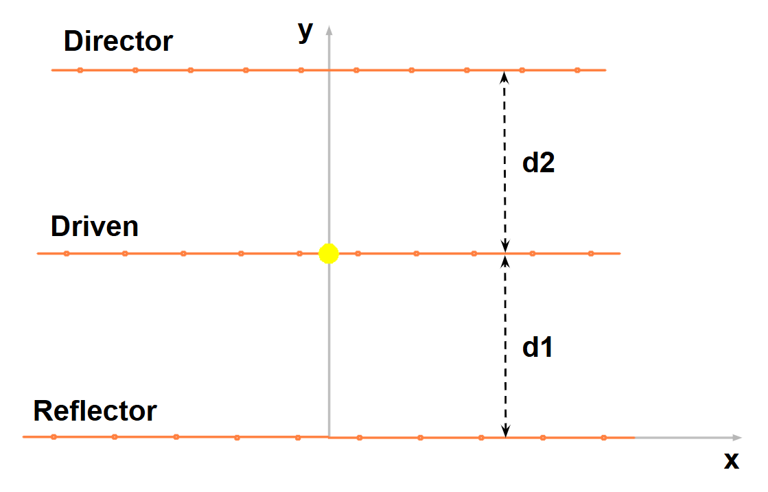
The modify_nec_file function defines a 3-element Yagi-Uda antenna (reflector, driven element, director) with dimensions normalized to 1 wavelength (λ) (λ ≈ 1 meter at 300 MHz). The antenna’s core geometry—including element lengths and radii—is fixed, while the spacings between elements (d₁: reflector-to-driven, d₂: driven-to-director) serve as the optimization variables. This normalization allows the design to be easily scaled to other frequencies by multiplying all dimensions by the desired wavelength.

As shown in Figure 2, the spacings d₁ (reflector-to-driven element) and d₂ (driven element-to-director) are the key optimization variables. The GA adjusts these spacings within practical bounds (0.1λ to 0.4λ) to explore performance trade-offs, simultaneously optimizing gain, VSWR, and front-to-back ratio through the cost function weights.

Genetic Algorithm Configuration and Execution

This final section of the script configures the GA’s optimization targets, search boundaries, and evolutionary parameters before launching the algorithm. Here’s how each component works:

VSWR0 = 1.1;   // Target VSWR
G0 = 9.0;      // Target gain in dBi
FBH0 = 15.0;   // Target F/B(H) in dB

VSWR_W = 80;  // VSWR weight %
G_W = 50;     // Gain weight %
FBH_W = 75;   // F/B(H) weight %

// Define bounds for d1 and d2
lower_bounds = [0.1; 0.1]; // Minimum spacing (meters)
upper_bounds = [0.4; 0.4]; // Maximum spacing (meters)

// GA parameters
pop_size = 10;   // Population size
max_gen = 3;     // Number of generations
crossover_rate = 0.7;
mutation_rate = 0.1;

ga_params = init_param();
ga_params = add_param(ga_params,"dimension",2);
ga_params = add_param(ga_params,"minbound",lower_bounds);
ga_params = add_param(ga_params,"maxbound",upper_bounds);

// Run the Genetic Algorithm
[optim_result, optim_cost] = optim_ga(antenna_cost, pop_size, max_gen, mutation_rate, crossover_rate, %T, ga_params);

antenna_cost(optim_result(1));

1. Target Definitions and Weighting

VSWR0 = 1.1;   // Ideal VSWR (perfect match = 1.0)
G0 = 9.0;      // Target gain (dBi)  
FBH0 = 15.0;   // Desired front-to-back ratio (dB)

VSWR_W = 80;   // Prioritizes VSWR (80% weight)
G_W = 50;      // Moderate gain emphasis  
FBH_W = 75;    // Strong focus on directivity

• Weight Rationale: The 80% VSWR weighting reflects typical design priorities where impedance matching is critical, while gain and FBH weights can be adjusted for specific applications.

2. Parameter Space Bounding

lower_bounds = [0.1; 0.1]; // Minimum element spacings (λ)
upper_bounds = [0.4; 0.4]; // Maximum spacings (λ)

• Practical Constraints: These bounds prevent unrealistic geometries (e.g., overlapping elements) while allowing sufficient exploration.

3. GA Evolutionary Parameters

pop_size = 10;       // 10 designs per generation
max_gen = 3;         // Evolution cycles (increase to 20-50 for final runs)
crossover_rate = 0.7; // 70% chance of trait mixing
mutation_rate = 0.1;  // 10% random parameter variation

ga_params = init_param();
ga_params = add_param(ga_params,"dimension",2); // d1 and d2 variables
ga_params = add_param(ga_params,"minbound",lower_bounds);
ga_params = add_param(ga_params,"maxbound",upper_bounds);

Population:

• Start small (10-20) for quick tests, scale to 20+ for production runs.

Crossover Rate (0.7)

• Purpose: Controls how often parent designs combine traits to create offspring.
• Mechanics: For each new design, there’s a 70% chance it inherits:
  • Spacing d₁ from Parent A and d₂ from Parent B (or vice versa).
• Trade-off: Higher values (>0.8) accelerate convergence but risk premature solutions.

Mutation Rate (0.1)

• Purpose: Introduces random variations to maintain diversity.
• Mechanics: Each optimized parameter (d₁, d₂) has a 10% chance to:
  • Randomize within bounds (e.g., d₁ = 0.15λ → 0.22λ).
• Trade-off: Lower values (<0.05) may stagnate; higher (>0.2) disrupts good designs.

Typical Tuning (For antenna problems):

• Initial Exploration: High mutation (0.15–0.2) + moderate crossover (0.6–0.7).
• Final Refinement: Reduce mutation (0.05–0.1) to fine-tune.

(Visual analogy: Crossover = “Antenna design inheritance”; Mutation = “Random component swaps”)

4. Optimization Launch

[optim_result, optim_cost] = optim_ga(antenna_cost, pop_size, max_gen, mutation_rate, crossover_rate, %T, ga_params);

• Outputs:
  • optim_result: Best-found parameters (d1, d2)
  • optim_cost: Final fitness value

5. Results Validation

antenna_cost(optim_result(1)); // Re-run and display optimal design

• Verification: Ensures the reported solution is reproducible and logs performance.

Key Recommendations:

1. For Initial Testing:
   • Use max_gen = 3-5 to verify the workflow (as shown)
2. Production Runs:
   • Increase to max_gen = 20-50, pop_size = 20-30
   • Log intermediate results to monitor convergence
3. Weight Adjustment:
   • If VSWR isn’t meeting targets, increase VSWR_W incrementally

Pro Tip:

Visualize population diversity by plotting parameter distributions across generations to detect premature convergence.

Conclusions and Next Steps

You now have a complete Genetic Algorithm optimizer ready for antenna design exploration. The provided GAoptimizer.sce script—paired with AN-SOF Engine’s simulation power—offers a turnkey solution to evolve high-performance antennas by automatically balancing gain, VSWR, and front-to-back ratio.

To get started immediately:

1. Download the scripts (includes NECcommands.sce and GAoptimizer.sce)
2. Run the workflow as-is to optimize the 3-element Yagi-Uda example
3. Tune weights (VSWR_W, G_W, FBH_W) for your specific requirements

Want to go further? Try:

• Adding more parameters (element lengths, wire radii) to the GA chromosome
• Experimenting with mutation rates (0.05–0.3) to escape local optima
• Combining with your measured data by modifying antenna_cost()

The real power of this approach lies in its adaptability—what will you optimize next?

See Also:

• AN-SOF Engine User Guide

• Nelder-Mead Optimization for Antenna Design Using the AN-SOF Engine and Scilab

• Building Effective Cost Functions for Antenna Optimization: Weighting, Normalization, and Trade-offs

---