Nelder-Mead Optimization for Antenna Design Using the AN-SOF Engine and Scilab

This article presents a Nelder-Mead optimization workflow for antenna design using AN-SOF Engine and Scilab. We demonstrate automated Yagi-Uda tuning via weighted cost functions, covering script implementation, NEC file modification, and result analysis for VSWR, gain, and front-to-back ratio optimization.

Optimization Fundamentals and the Nelder-Mead Method

Since the release of the AN-SOF Engine as a standalone console application, users gain enhanced flexibility in running simulations independently of the AN-SOF graphical user interface (UI). This capability enables direct integration of the AN-SOF calculation engine into third-party software or custom algorithmic workflows. Before proceeding with this tutorial, we recommend reviewing the AN-SOF Engine User Guide for foundational knowledge.

What is an Antenna Optimizer?

An optimizer is a computational tool designed to determine the extreme value (maximum or minimum) of an output parameter by systematically varying input variables in an antenna design. For example, typical optimization goals include maximizing gain or minimizing VSWR in a transmitting antenna. Since finding a maximum can be redefined as an equivalent minimum-search problem (e.g., maximizing G ≡ minimizing −G), optimization tasks are generally framed as minimization problems.

Minima can be classified as global (the absolute lowest value across the entire parameter space) or local (the lowest value within a limited subset of parameters), as illustrated in Fig. 1. A brute-force approach—evaluating every possible point along the parameter axis—would guarantee identification of the global minimum but is computationally prohibitive, especially in multidimensional problems where multiple input variables (e.g., antenna dimensions, feed positions) and output objectives (e.g., gain, bandwidth, efficiency) must be considered simultaneously.

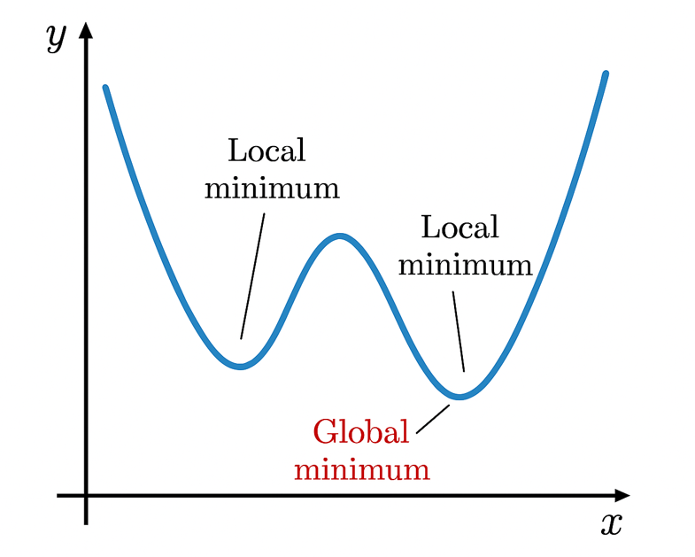
Instead, efficient optimization methods begin at an initial guess, ideally near a minimum. However, a key challenge is avoiding convergence to a local minimum—a suboptimal solution that appears adequate but fails to achieve the best possible performance. Consequently, successful optimization often involves iterative refinement and heuristic adjustments to balance computational cost with solution quality, ultimately arriving at a design that meets the desired criteria.

Optimization Methods and the Role of Cost Functions

Optimization encompasses a wide array of methods, most of which rely on defining a cost function—a mathematical construct that quantifies the relative importance of each output parameter in the optimization process. Given the diversity of available techniques and the need to tailor the cost function to specific design goals, the AN-SOF Engine is designed for seamless integration with custom optimization algorithms, ensuring adaptability to unique requirements.

Among the simplest and most widely used approaches is the Nelder-Mead method, a gradient-free optimization technique that iteratively refines a simplex (a geometric shape defined by n+1 vertices in n-dimensional space) to converge toward a minimum. By evaluating and comparing the cost function at each vertex, the method adaptively adjusts the simplex through operations like reflection, expansion, and contraction, balancing exploration of the parameter space with convergence efficiency.

In this guide, we demonstrate how to implement a Nelder-Mead optimizer using Scilab, a free and open-source alternative to MATLAB. Scilab was selected for its versatility and accessibility, though the provided scripts can be adapted to other programming languages, provided a compatible Nelder-Mead algorithm is available.

Implementing a Nelder-Mead Optimizer for AN-SOF: Script Walkthrough

To streamline your workflow, this guide provides a ready-to-use optimization template rather than building a script from scratch. The AN-SOF Engine utilizes antenna description files in .nec format, and we include a complementary script containing all NEC commands supported by AN-SOF.

Prerequisites:

1. Before running the optimizer, execute the provided NECcommands.sce script to load the necessary command functions into the Scilab environment.
2. For users unfamiliar with NEC syntax, we recommend reviewing the AN-SOF Engine User Guide and Importing Wires Guide for comprehensive command references.

Download Resources:

(Includes both NECcommands.sce and NelderMeadOptimizer.sce files)

The following sections will dissect the NelderMeadOptimizer.sce code structure, explaining its key components and their roles in the optimization process.

Optimization Example: Yagi-Uda Antenna Design

Our demonstration focuses on optimizing a 3-element Yagi-Uda antenna in free space, operating at 300 MHz. At this frequency, the wavelength is approximately 1 meter (0.999 m, rounded for practical purposes), simplifying the problem into normalized dimensions. This normalization allows for straightforward rescaling—multiplying all antenna dimensions by the desired wavelength—to adapt the design to other frequencies.

Optimization Objectives

The goal is to achieve specific target values for three key performance metrics:

• VSWR₀ = 1.1 (voltage standing wave ratio)
• G₀ = 9 dBi (gain)
• FBH₀ = 15 dB (horizontal front-to-back ratio)

Rather than simply minimizing these parameters, the optimizer aims to converge toward these predefined targets. To quantify deviations from the targets, we define the following normalized error terms:

• ΔVSWR = |VSWR − VSWR₀| / VSWR₀
• ΔG = |G − G₀| / G₀
• ΔFBH = |FBH − FBH₀| / FBH₀

While this formulation uses absolute errors, alternative approaches (e.g., squared errors) could also be employed. This flexibility underscores the importance of tailoring the cost function to the specific problem requirements.

Cost Function Construction

A naive cost function might sum all deviations equally:

cost = ΔVSWR + ΔG + ΔFBH

However, this approach assigns equal weight to each parameter, which may not reflect practical priorities. For instance, achieving optimal VSWR (critical for impedance matching) might warrant greater emphasis than gain or directivity. To address this, we introduce a weighted cost function:

cost = (VSWR_W · ΔVSWR + G_W · ΔG + FBH_W · ΔFBH) / (VSWR_W + G_W + FBH_W)

Here, VSWR_W, G_W, and FBH_W represent the relative importance of each deviation. The denominator normalizes the cost, enabling interpretation of weights as percentages:

• VSWR_W = 80 (80% priority)
• G_W = 50 (50% priority)
• FBH_W = 75 (75% priority)

This weighted framework ensures the optimizer prioritizes VSWR matching while still accounting for gain and front-to-back ratio, aligning with typical design trade-offs in antenna engineering.

Implementation of the Cost Function in Scilab

The provided antenna_cost(x) function implements our weighted optimization strategy while handling simulation workflow and error management: 

function cost=antenna_cost(x)

// Access global file paths
global nec_filename results_csv log_csv;
// Access global target values
global VSWR0 G0 FBH0;
// Access global weigths
global VSWR_W G_W FBH_W;

// Element spacings
d1 = x(1);
d2 = x(2);

global trial_count;
trial_count = trial_count + 1;

// Modify the .NEC file with new values
modify_nec_file(nec_filename, d1, d2);

// Run AN-SOFengine.exe
dos('start /wait /min C:\AN-SOFengine\AN-SOFengine.exe');

// Read output gain from CSV
[vswr, gain, fbh] = read_antenna_results(results_csv);

if isempty(vswr) | isnan(vswr) | ...
isempty(gain) | isnan(gain) | ...
isempty(fbh)  | isnan(fbh) then
trial_count = trial_count - 1;
cost = 1e6; // A large penalty value so optimizer discards this trial
return;
end

// Display valid results
disp(msprintf("%4d  | %5.4f | %5.4f | %5.2f | %5.2f | %5.2f", ... 
trial_count, d1, d2, vswr, gain, fbh));

// Append results to CSV file
fid = mopen(log_csv, "at"); // Open in append mode
mfprintf(fid, "%d,%5.4f,%5.4f,%5.2f,%5.2f,%5.2f\n", ...
trial_count, d1, d2, vswr, gain, fbh);
mclose(fid);

// Cost function: Minimize weighted relative error
cost = (VSWR_W* abs(vswr - VSWR0)/VSWR0 + ...
G_W* abs(gain - G0)/G0 + ...
FBH_W* abs(fbh - FBH0)/FBH0) / ...
(VSWR_W + G_W + FBH_W);

endfunction

Here’s how it operates:

The function begins by accessing global variables containing file paths (nec_filename, results_csv, log_csv), target values (VSWR0, G0, FBH0), and optimization weights (VSWR_W, G_W, FBH_W). These globals ensure consistency across multiple function calls during the optimization process.

Two key operations occur with each function evaluation:

1. Geometry Update: The Yagi-Uda element spacings (d1, d2) from the optimization vector x are written to the NEC file via modify_nec_file()
2. Simulation Execution: The AN-SOF engine is called to compute the antenna performance

Robust error handling is implemented:

• If results are invalid (empty/NaN), the function returns a large penalty value (1e6), forcing the optimizer to discard this trial
• Valid results are both displayed in the console and appended to a CSV log file for record-keeping

The core optimization occurs in the final calculation, where the weighted cost is computed as:

cost = ( VSWR_W * abs(vswr – VSWR0) / VSWR0 + …

G_W * abs(gain – G0) / G0 + FBH_W * abs(fbh – FBH0) / FBH0 ) / ( VSWR_W + G_W + FBH_W )

This implementation efficiently combines:

• Automated NEC file modification
• AN-SOF simulation triggering
• Result validation and logging
• Weighted cost calculation

The trial counter (trial_count) provides visibility into the optimization progress, with each valid evaluation generating a console output and CSV record showing the iteration number, spacings, and resulting antenna parameters.

Geometry Modification Function

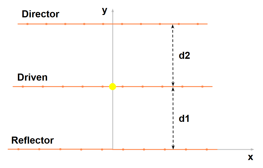
The modify_nec_file function dynamically updates the antenna geometry in the .nec file at each optimization step. It takes three inputs: the target filename (filename) and the two variable spacings (d1, d2), which represent (see Fig. 2):

• d1: Reflector-to-driven-element spacing
• d2: Driven-element-to-director spacing

function modify_nec_file(filename, d1, d2)
Seg = 7; // Number of segments per element

antenna = [
GW(1, Seg, -0.25, 0, 0, 0.25, 0, 0, 0.001)
GW(2, Seg, -0.238, d1, 0, 0.238, d1, 0, 0.001)
GW(3, Seg, -0.226, d1+d2, 0, 0.226, d1+d2, 0, 0.001)
GE(0)
FR(0, 1, 300, 0.0)
EX(0, 2, (Seg+1)/2, 1.4142136, 0)
RP(37, 73, 0, 0, 5, 5, 1)
];

// Write modified .NEC file
mputl(antenna, filename);
endfunction

NEC Command Implementation

The function constructs the antenna model using standard NEC commands stored in the antenna array:

• GW: Defines wire geometries for each element (reflector, driven element, director) with:
  • Fixed lengths (-0.25 to 0.25 for reflector, scaled for other elements)
  • Positions adjusted by d1 and d2
  • Uniform wire radius (0.001 m)
• GE: Specifies free-space conditions (no ground plane)
• FR: Sets the operating frequency (300 MHz)
• EX: Excites the driven element at its center (segment (Seg+1)/2) with a voltage source
• RP: Sets the radiation pattern angular resolution (37 × 73)

The mputl function writes these commands to the specified .nec file, which AN-SOF reads for simulation.

Segment Density Consideration

While this example uses only 7 segments per element for simplicity, practical designs require convergence testing. Empirical comparisons with measured VSWR data suggest 20–50 segments per element are typically needed for accuracy. Note that the driven element’s segment count (Seg) must be odd to ensure the excitation source aligns with its geometric center.

This function exemplifies how optimization parameters (d1, d2) are translated into physical geometry changes, enabling systematic performance improvements.

Result Extraction Function

The read_antenna_results function retrieves key antenna performance metrics from the CSV output file generated by the AN-SOF Engine after each simulation. This function accepts the filename as input and returns the performance parameters we are interested in:

• VSWR (voltage standing wave ratio)
• Gain (in dBi)
• Front-to-back ratio in the horizontal plane (FBH)

function [vswr, gain, fbh]=read_antenna_results(filename)

// Read CSV file
[data, c] = csvRead(filename, ';', [], [], [], [], [], 3);

// VSWR is in the 7th column
vswr = data(1, 7);

// Gain is in the 10th column
gain = data(1, 10);

// F/B(H) is in the 15th column
fbh = data(1, 15);

endfunction

The function uses Scilab’s csvRead utility to parse the output file, which is formatted with semicolon (;) delimiters. Specific columns are indexed to extract the relevant data:

• Column 7: Contains the VSWR value
• Column 10: Stores the antenna gain
• Column 15: Holds the horizontal front-to-back ratio

These column positions correspond to the standardized output format of the AN-SOF Engine, which appends a “_Results.csv” suffix to the project name for each simulation run.

This function bridges the simulation and optimization processes by:

1. Automatically reading the latest results after each AN-SOF execution
2. Providing the cost function with updated performance metrics
3. Enabling real-time evaluation of antenna parameter variations

The extracted values feed directly into the cost calculation, driving the optimizer toward the target specifications. For further details on the CSV structure or output options, consult the AN-SOF Engine User Guide.

Optimization Setup and Execution

This concluding portion of the script establishes the framework for running the antenna optimization: 

// Define file paths
nec_filename = "C:\AN-SOF\yagi3.nec";
results_csv = "C:\AN-SOF\yagi3_Results.csv";
log_csv = "C:\AN-SOF\optimizer_log.csv"; // CSV log file for trial results

// Set directory for AN-SOFengine.exe
chdir("C:\AN-SOFengine\");

// Display table header with trial results
disp("Trial |   d1   |   d2   |  VSWR | G(dBi)| F/B(H)");
disp("------------------------------------------------");
fid = mopen(log_csv, "wt");
mfprintf(fid, "Trial,d1,d2,VSWR,Gain(dBi),F/B(H)\n");
mclose(fid);

// Define target values and weights
global VSWR0 G0 FBH0;
global VSWR_W G_W FBH_W;

VSWR0 = 1.1;   // Target VSWR
G0 = 9.0;      // Target gain in dBi
FBH0 = 15.0;   // Target F/B(H) in dB

VSWR_W = 80;  // VSWR weight %
G_W = 50;     // Gain weight %
FBH_W = 75;   // F/B(H) weight %

// Set initial values for [d1, d2]
x0 = [0.15, 0.2]; // Initial guess for element spacings

// Optimization parameters
options = optimset("MaxIter", 50, "MaxFunEvals", 50, ...
                   "TolFun", 1e-2, "TolX", 1e-2);

// Run Nelder-Mead optimization
optim_result = fminsearch(antenna_cost, x0, options);

// Display optimized results
antenna_cost(optim_result);

It performs several key functions:

File Path Configuration

The script begins by defining essential file paths: the input NEC file (yagi3.nec), the results file generated by AN-SOF (yagi3_Results.csv), and a dedicated log file (optimizer_log.csv) that records all trial results. The working directory is set to the AN-SOF Engine installation folder to ensure proper execution.

Results Logging Initialization

A formatted header is created for both the console display and the log file, clearly labeling each column (Trial, d1, d2, VSWR, Gain, and F/B(H)) to maintain organized data tracking throughout the optimization process.

Target Parameters and Weighting

The script declares global variables for:

• Target values: VSWR (1.1), Gain (9 dBi), and Front-to-Back Ratio (15 dB)
• Optimization weights: VSWR (80%), Gain (50%), and F/B(H) (75%)
  These weights reflect the relative importance of each parameter in the cost function, prioritizing impedance matching (VSWR) while still considering radiation characteristics.

Optimization Configuration

The process begins with an initial guess for element spacings (d1 = 0.15m, d2 = 0.20m) and sets key optimization parameters:

• Maximum iterations and function evaluations (50 each)
• Convergence tolerances (1% for both function value and parameters)

Optimization Execution

The core optimization is performed using Scilab’s fminsearch function, which implements the Nelder-Mead algorithm. This function repeatedly calls the antenna_cost function, adjusting the element spacings (d1, d2) to minimize the weighted cost.

Results Display

Finally, the optimized parameters are passed to the cost function one last time to display the best-found solution in the console and record it in the log file.

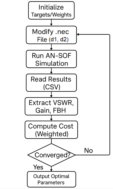
This complete implementation demonstrates a practical workflow for antenna optimization (see Fig. 3), combining file management, parameter definition, algorithm configuration, and results tracking into a cohesive automated process.

Summary & Demonstration

This guide has presented a complete framework for optimizing antenna designs using the AN-SOF Engine and Scilab. We covered:

1. Optimization Fundamentals – The role of cost functions, weighted objectives, and the Nelder-Mead method for gradient-free parameter tuning.
2. Implementation – A ready-to-use Scilab template integrating AN-SOF simulations, including:
   • Dynamic NEC file modification (modify_nec_file)
   • Automated result extraction (read_antenna_results)
   • Weighted cost function construction
3. Workflow Automation – File handling, target specification, and iterative optimization with convergence controls.

To see this process in action, watch the demonstration below, where we optimize the 3-element Yagi-Uda antenna in real time:

The video showcases:

• Live updates of antenna parameters (VSWR, gain, F/B) across iterations
• Convergence behavior of the Nelder-Mead algorithm
• Final optimized geometry and its radiation characteristics

This approach can be adapted to other antenna types or optimization goals by modifying the cost function and NEC geometry. For advanced users, the framework supports integration with machine learning libraries or multi-objective optimization schemes.

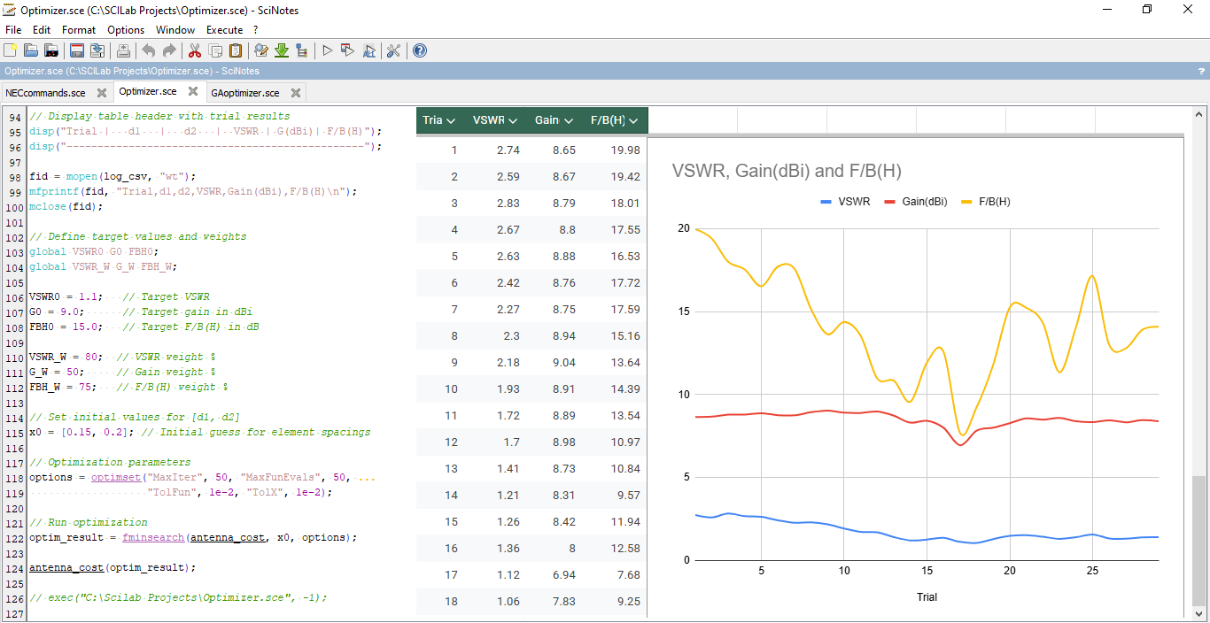
The log file (specified by log_csv) provides critical optimization tracking by recording all trial parameters and results. This enables post-processing visualization of convergence behavior, such as plotting VSWR, gain, and F/B (H) versus trial count (Fig. 4), revealing trends toward target values and algorithm efficiency.

As detailed in the AN-SOF Engine User Guide, the engine generates both a results CSV file and native project files (.emm, .wre, .cur, .the, .phi, .pwr). These outputs enable seamless transition to the AN-SOF UI, where users can analyze the optimized model from the final iteration.

Next Steps:

• Experiment with different weights or target values
• Extend the script to optimize additional parameters (e.g., element lengths)
• Validate results with experimental measurements

For advanced customization and detailed command references, consult the AN-SOF Engine User Guide.