Search for answers or browse our Knowledge Base.
Guides | Models | Validation | Book
Understanding the Antenna Near Field: Key Concepts Every Ham Radio Operator Should Know
Learn the essentials of the antenna near field! This guide explains key concepts for ham radio operators, from reactive fields to EMF safety, helping you better understand antenna radiation and ensure compliance. Ideal for both beginners and experienced hams alike!
Introduction: Demystifying the Near Field of Antennas for Ham Radio Enthusiasts
For ham radio operators and those venturing into the world of antennas, terms like near field and far field often arise in discussions about antenna performance and electromagnetic radiation. But what do these terms truly mean, and why are they important? This article aims to provide a clear and accessible explanation of these concepts, avoiding complex equations or advanced physics.
The near field is a crucial region surrounding an antenna where electromagnetic fields exhibit unique behaviors distinct from those in the far field. A solid understanding of this region is vital not only for optimizing antenna performance but also for ensuring compliance with electromagnetic field (EMF) safety standards, a key consideration for safe operation. While a comprehensive understanding of antenna theory involves Maxwell’s equations and advanced mathematical analysis (as detailed in authoritative texts like Antennas by John D. Kraus), this article focuses on conveying the fundamental principles in a straightforward manner. Whether you are new to ham radio or seeking to enhance your conceptual knowledge, this guide will help you grasp the essentials of near field, far field, and wave propagation in a practical and approachable way.
Understanding the Near-Field Region: A Conceptual Overview
When transmitting a signal using your ham radio, the antenna serves as the critical interface between your radio and the surrounding space, radiating electromagnetic energy into the air. But what occurs in the immediate vicinity of the antenna? This is where the near-field region becomes significant—a complex yet fascinating area essential to understanding antenna operation.
Energy Flow from Radio to Antenna
Antennas, often referred to as aerials, are typically fed by transmission lines such as open-wire lines or coaxial cables. These lines deliver radio frequency (RF) power from your radio to the antenna. In an ideal scenario—where the antenna is perfectly matched to the transmission line and losses are negligible—all the power supplied to the line reaches the antenna’s feedpoint. From this point, the process of energy transformation and radiation begins.
At the antenna’s feedpoint, electromagnetic energy is released into the surrounding space, establishing a distribution of electric (E) and magnetic (H) fields. This process creates a current distribution along the antenna’s metallic structure, which in turn generates these fields around the antenna. These fields are fundamental to the propagation of your signal through space.
The Interaction of Electric and Magnetic Fields
The behavior of the fields near the antenna is intricate. Electric field lines originate perpendicularly from regions of the antenna with a positive charge and terminate at areas with a negative charge. Since RF signals oscillate with time, the currents, charges, and both electric and magnetic fields fluctuate in sync. This oscillation enables your signal to carry information across distances.
Magnetic fields, however, exhibit a different behavior. Unlike electric fields, which begin and end at specific points, magnetic field lines form continuous loops around the antenna. To visualize this, consider a simple half-wave dipole antenna (Figure 1). The electric field lines radiate outward, while the magnetic field lines encircle the antenna in closed loops.

Stored Energy in the Near Field
A defining characteristic of the near-field region is its ability to store energy. This energy exists in two distinct forms:
- Electric Energy: Associated with the electric field lines.
- Magnetic Energy: Associated with the magnetic field lines.
To better understand this, the near field can be likened to an electric circuit. The electric energy is analogous to the energy stored in a capacitor (C), while the magnetic energy resembles the energy stored in an inductor (L). When these components are combined in an LC circuit, their energies interact. If the electric and magnetic energies are equal, the system achieves resonance, and the reactances cancel each other out. This does not imply the absence of energy—rather, the energies are balanced.
For instance, in a half-wave dipole antenna, the feedpoint reactance is typically positive, indicating that magnetic energy dominates over electric energy. Nevertheless, both forms of energy coexist in the space surrounding the antenna, interacting in a precise balance that facilitates effective signal propagation.
The LC Oscillator Bubble: The Heart of the Near-Field Region
To fully comprehend the near-field region of an antenna, it is helpful to conceptualize it as an LC oscillator bubble. This bubble represents the space surrounding the antenna where electromagnetic energy is stored and exchanged between electric and magnetic fields, akin to the energy exchange in an inductor-capacitor (LC) circuit. Let’s explore this concept in detail.
What is the LC Oscillator Bubble?
The near-field region is characterized by the concentration of the antenna’s reactive fields—the electric and magnetic fields. These fields are tightly bound to the antenna’s structure and do not extend far into the surrounding space. The electric field lines are anchored to the antenna’s metallic surface, originating from areas of positive charge and terminating at regions of negative charge. Simultaneously, the magnetic field lines form closed loops around the antenna, linked to the currents flowing through its structure.
This interplay of electric and magnetic fields creates a dynamic energy exchange. Electric energy transforms into magnetic energy, and vice versa, oscillating at the frequency of the RF signal. In essence, the near-field region is an extension of the antenna itself, where the antenna’s materials define the boundaries of these electromagnetic fields. This region acts like an invisible bubble, storing and cyclically transforming energy, much like an LC circuit.
Accounting for the Radiated Power
While the LC oscillator bubble provides a useful framework for understanding the near-field region, it does not fully capture the antenna’s function. Antennas are designed to radiate power, and this radiated power escapes the LC oscillator bubble, propagating outward into space. From the perspective of the antenna’s feedpoint, this radiated power is represented by the resistive component of the antenna’s input impedance.
However, not all the power delivered to the antenna is radiated. A portion is lost as heat due to the resistance of the antenna’s metallic structure, a phenomenon known as skin effect losses. To complete the picture, two types of resistance must be considered:
- Radiation Resistance: This represents the power successfully radiated into space.
- Loss Resistance: This accounts for the power dissipated as heat in the antenna’s conductors.
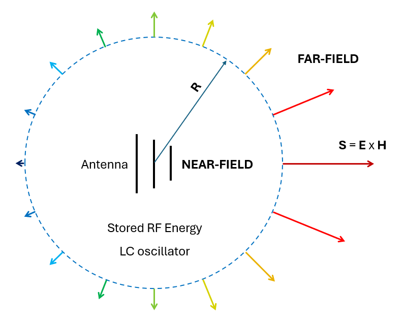
Figure 2 depicts how the radiated power density propagates beyond the LC oscillator bubble as a Transverse Electromagnetic (TEM) wave. This wave carries energy away from the antenna, and its power density is described by the Poynting vector (S). (The Poynting vector can be thought of as the directional flow of electromagnetic energy, analogous to the way sunlight carries energy to warm the Earth’s surface.)
Transitioning to the Far-Field Region
Beyond the LC oscillator bubble lies the far-field region. Here, the radiated wave fully detaches from the antenna and propagates as a self-sustaining TEM wave. In the far field, the electric (E) and magnetic (H) fields oscillate in phase, are perpendicular to each other, and are also perpendicular to the direction of wave propagation, as indicated by the Poynting vector.
In this region, the wavefront becomes spherical, and the fields no longer depend on the antenna’s structure. The electric field lines close on themselves, and the magnetic field lines are no longer tied to the antenna’s currents. Instead, the wave sustains itself through the mutual generation of electric and magnetic fields—each field creating the other as the wave propagates through space.
Power Density vs. Radiated Power: Understanding the Distinction
When analyzing antennas and electromagnetic waves, it is essential to differentiate between power density and radiated power. While these concepts are interrelated, they describe distinct aspects of how energy propagates from an antenna. Let’s examine this distinction in detail.
Power Density in the Far Field
In the far-field region, the electromagnetic wave radiated by the antenna propagates outward, and its electric (E) and magnetic (H) fields weaken as they travel. Specifically, the fields attenuate according to the inverse distance law: doubling the distance from the antenna reduces the field strength to half its original value.
Power density, represented by the Poynting vector (S), quantifies the energy flow per unit area and is calculated by multiplying the E and H fields. Its units are Watts per square meter (W/m²). Power density follows the inverse square law: doubling the distance from the antenna reduces the power density to one-fourth of its original value. This occurs because the energy spreads over a larger wavefront area as the wave propagates.
For example, consider the sun radiating energy. At Earth’s surface, after accounting for atmospheric absorption and scattering, we receive approximately 1,000 W/m2 on a clear day. If you had a 1 m2 solar cell with 100% efficiency, oriented perpendicularly to the incoming sunlight, it would collect 1,000 Watts of power. Doubling the solar cell’s area to 2 m2 would yield 2,000 Watts. This example highlights the importance of distinguishing between power density, measured in Watts per square meter (W/m2), and power, measured in Watts (W), which represents the total energy received by the solar cell.
Similarly, in the context of antennas, we must not confuse the power density, represented by the Poynting vector radiating from a transmitting antenna, with the radiated power. Radiated power is calculated by integrating the power density over a spherical wavefront—essentially summing the power density contributions across each square meter of the sphere’s surface. This distinction is crucial for understanding how energy propagates from an antenna and how it is measured in both near-field and far-field regions.
Power Density in the Near Field
The concept of power density also applies in the near-field region, but the situation is more complex. Inside the “LC oscillator bubble,” the fields remain concentrated around the antenna, and the energy exchange between electric and magnetic fields dominates. If a receiving antenna is placed in the near-field region of a transmitting antenna, it becomes part of the transmitting antenna’s electromagnetic environment.
In this scenario, the receiving antenna does not simply capture power density as it would in the far field. Instead, it interacts with the transmitting antenna through induction, creating a current distribution in the receiver. This interaction makes near-field calculations significantly more challenging, as the fields are non-uniform and depend on the specific geometry and placement of the antennas.
Radiated Power: The Broader Perspective
Radiated power refers to the total energy that escapes the antenna and propagates into space. It represents the power that ultimately reaches the far field and can be received by distant antennas. However, a distant receiving antenna will not capture the total radiated power but only a fraction of it. This fraction is determined by multiplying the power density at the receiver’s location by the antenna’s effective area, much like calculating the power received by a solar cell based on the power density of sunlight at its location.
That said, not all the power delivered to a transmitting antenna is radiated. Some is lost as heat due to the resistance of the antenna’s conductors (skin effect or ohmic losses). Understanding these losses is essential for optimizing antenna efficiency and ensuring effective energy transfer.
To summarize:
- Power Density (S): Describes the energy flow per unit area (W/m²) and follows the inverse square law with distance in the far field.
- Radiated Power: Represents the total power that escapes the antenna and propagates into space, accounting for losses in the antenna’s structure. Unlike power density, the radiated power, measured in Watts, remains constant regardless of distance (principle of energy conservation).
Calculating the Near Field in AN-SOF
To calculate the near field in AN-SOF, you must first define a grid of points in space where the electric (E), magnetic (H), and power density (S) fields will be computed. To set up the grid for the near field, navigate to the Setup tab > Near Field panel. Here, you’ll find three coordinate system options: Cartesian, Cylindrical, and Spherical.
For a transmitting antenna positioned above a ground plane, the near field at ground level as a function of distance from the antenna is often of particular interest. To analyze this, select the Spherical option and set Theta = 90° (ground level). The angle Phi (azimuth) indicates the direction on the xy-plane, starting from Phi = 0° at the x-axis and increasing to Phi = 90° at the y-axis, Phi = 180° at the -x axis, Phi = 270° at the -y axis, and returning to the positive x-axis at Phi = 360° (which coincides with Phi = 0°).
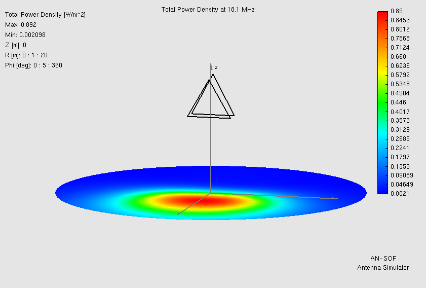
After specifying the observation direction, you can set the range for the distance R from the antenna. As a practical example, Figure 3 shows the power density as a function of distance in the direction of maximum radiation (where the main lobe points in the far-field region) for a 17m band delta loop beam. The details of the model can be found in the following articles:

Figure 3 illustrates the power density, which peaks near the antenna and then decays following the inverse square law with distance. In this model, the input power to the feeder is set to 100 W, with 84.6 W delivered to the antenna feedpoint at the resonant frequency and 15.4 W lost in the feeder. By navigating to the Results menu > Power Budget, you can see that the radiated power is 62.1 W. The difference between the antenna input power (84.6 W) and the radiated power represents the power lost as ohmic losses in the antenna structure and as heat in the ground plane below the antenna. As explained earlier, the radiated power remains constant across all field regions (principle of energy conservation), while the power density, as illustrated in Figure 3, varies with distance.
Insights on the Boundary Between the Near and Far Field Regions
At this point, we recognize that the near-field region is characterized by electric and magnetic field lines closely linked to the antenna’s metallic structure, where energy is stored in the electric and magnetic fields. But how far does this region extend? This question has been a long-standing topic of discussion and continues to generate debate among RF professionals.
There is no abrupt boundary between the near and far field regions; instead, the near electromagnetic field gradually transforms into a TEM wave as distance from the antenna increases. Traditional formulas, which remain widely accepted, are still published in antenna textbooks. An online calculator implementing these formulas is available at this link:
Antenna Near – Far Field Boundary Calculator
A more accurate method to determine the practical boundary between field regions is based on the concept of wave impedance, defined as the ratio between the electric (E) and magnetic (H) fields. In the far-field region, the wave impedance approaches 377 Ohms for a TEM wave propagating in free space. Thus, the onset of the far field can be identified when the wave impedance consistently reaches 377 Ohms within a given margin of error.
In AN-SOF, the wave impedance (Zw) is calculated alongside the power density, as well as a parameter called the Wave Matching Coefficient (WMC). The WMC, expressed in decibels, is analogous to the return loss in a transmission line and measures the mismatch between the actual wave impedance and 377 Ohms. To access the power density (S), Zw, and WMC, navigate to the AN-SOF main menu > Results > List Power Density Pattern (fixed frequency, varying point coordinates) or List Power Density Spectrum (fixed point coordinates, varying frequency).
Using the WMC provides a straightforward way to determine the boundary between the near and far field regions. When the WMC exceeds 20 dB, it indicates that we are in the far-field region.
Frequently Asked Questions About the Near Field of Antennas
Now that we’ve explored the conceptual framework of the near-field and far-field regions, let’s address some common questions from the ham radio community.
1. If the power density in the near field is stronger than predicted by the inverse-square law, doesn’t that violate the conservation of energy?
This question stems from a common confusion between power (measured in Watts) and power density (measured in Watts per square meter). In the near-field region, the power density is indeed stronger than in the far field and does not follow the inverse-square law. This is because the electric (E) and magnetic (H) fields are significantly more intense close to the antenna.
However, this does not imply a violation of energy conservation. The near-field power density includes reactive components—parts of the fields associated with stored energy rather than radiated power. These reactive components oscillate locally, creating strong fields near the antenna, but they do not contribute to energy propagation. When you calculate the total radiated power by integrating the power density over a sphere surrounding the antenna, the result remains constant, regardless of the sphere’s size. This consistency is a direct consequence of the conservation of energy: energy is neither created nor destroyed; it is simply distributed differently between the near and far fields.
2. If the electromagnetic wave in the near field isn’t a Transverse Electromagnetic (TEM) wave, how can a receiver pick up a signal when placed close to a transmitting antenna?
A common misconception is that only TEM waves can induce signals in a receiver. While TEM waves dominate in the far field, the near field operates differently. In the near-field region, the electric and magnetic fields do not form a perfect TEM wave, but they still interact with a receiving antenna through induction.
When a receiving antenna is placed in the near field, the oscillating electric and magnetic fields induce currents in its structure. These currents generate a voltage and current at the receiver’s terminals, enabling it to detect the signal. This process does not require a TEM wave; instead, it relies on the coupling between the fields and the receiver’s conductive elements. Thus, even though the near-field wave is not TEM, it can effectively transfer energy to a nearby receiver.
3. If the near field is such a concern, shouldn’t cellular phones—which operate at microwave frequencies and are held close to the brain—be banned? Why do ham radio operators need to worry about EMF compliance?
This is a valid point, and it’s important to note that cellular phones are subject to stringent EMF compliance regulations in most countries. These regulations ensure that the electric (E), magnetic (H), and power density (S) fields emitted by phones remain below established safety limits to protect users from potential health risks.
For ham radio operators, EMF compliance is equally critical, particularly when transmitting at high power levels. The near-field region is where field strengths are highest, and prolonged exposure to strong fields can pose health hazards. By understanding and adhering to EMF safety guidelines, ham radio operators can ensure their activities are safe for themselves and those around them.
The primary factor influencing field strength is transmit power: higher power levels result in stronger fields. By calculating field levels and ensuring they remain below safety thresholds, operators can enjoy their hobby responsibly. Tools such as field strength meters, compliance calculators, and antenna simulations can assist in this process.
Why Is the Near Field Important for Ham Radio Operators?
Understanding the near field is crucial for ham radio operators because it directly impacts antenna performance, safety, and operational efficiency. This region, where electromagnetic energy is stored and exchanged between electric and magnetic fields, influences key factors such as impedance matching and radiation efficiency. Additionally, the near field is where electromagnetic field (EMF) strengths are highest, making it essential to assess and manage exposure levels to comply with safety standards, especially when transmitting at high power.
The near field also affects how antennas interact with their environment, including nearby objects and other antennas. This knowledge helps operators minimize interference and maximize performance in complex setups. In short, mastering the near field enables ham radio enthusiasts to enhance their technical skills, ensure safe operation, and achieve better results in their radio communications.
