Element Spacing Simulation Script for Yagi-Uda Antennas

Introduction

Scilab > is a free and open source software platform for numerical computation. It is one of the most suitable tools to create scripts that allow us to run multiple simulations in AN-SOF.

This guide explains how to run a script in Scilab to simulate a 3-element Yagi-Uda antenna and get the results as a function of the spacing between the elements. A second script allows us to plot the antenna gain versus element spacing. The scripts can be easily extended for any number of elements as well as to obtain another output parameter, other than the gain, simply by reading the output files returned by the simulation.

Download and install Scilab

Download Scilab from the following link:

https://www.scilab.org/download/

There are 32 and 64 bits versions.

We recommend installing Scilab on the same machine as AN-SOF or creating a shared folder where Scilab saves the files with the antenna descriptions and from where AN-SOF, in turn, can read these files.

Running the Scilab scripts and AN-SOF

Download the Scilab scripts from this link,

https://antennasimulator.com/examples/AN-SOF_Scripts_Yagi_Spacing.zip

Unzip the files and open them with Scilab.

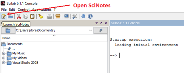
There is a text editor called SciNotes that you can use to open scripts with extension sce.

There are two scripts for this project, namely, “yagi_spacing.sce” and “yagi_spacing_gain.sce”.

yagi_spacing.sce

It generates multiple files with extension .nec. Each file contains a description in NEC format of a 3-element Yagi-Uda antenna. The output files from this script will have varying names according to the element spacing. Pay attention to the following line:

// Output files with varying names according to element spacing

    mputl(yagi,'C:/AN-SOF/yagi_spacing' + string(i) + '.nec');

which declares the directory where the output files of this script will be saved. Create the folder C:/AN-SOF/ to use the script as is or use any folder you like, but modify this line to declare your own directory.

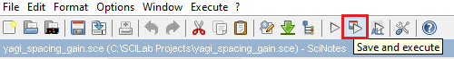
To run the script, go to the SciNotes toolbar and click on the “Save and execute” button (or you can also press F5 on the keyboard).

After executing the script, check that the files yagi_spacing15.nec to yagi_spacing30.nec have been generated in the chosen directory. The names of these files correspond to the range of variation of the element spacing (“15” means 0.15 meters, “16” means 0.16 meters and so on). To change this range, modify this line,

dy = (0.15:0.01:0.3)';  // Varying element spacing

Now you can go to AN-SOF and run the bulk simulation of the generated NEC files. Go to the AN-SOF main menu > Simulate > Run Bulk Simulation. A message will appear asking if you want to save the changes in the current project, since the bulk simulation requires closing the project that is currently open. Then, a dialog box will be displayed where a directory and the input .nec files can be selected.

Select all the files, from yagi_spacing15.nec to yagi_spacing30.nec, in the C:\AN-SOF\ directory or in the directory you have created. Then, click on the “Open” button and the bulk simulation will begin. The input files will be imported and computed one after another in alphabetical order.

Once AN-SOF has completed the simulation, you will find the output files with results in the same directory where the .nec files are, that is in C:\AN-SOF if you did not modify the script.

As an example, for the input file “yagi_spacing15.nec”, the following files will be generated:

Files of the AN-SOF project

yagi_spacing15.emm > main file of the project (it can be opened with AN-SOF)

yagi_spacing15.wre > geometry data (wires, segments, connections)

yagi_spacing15.txt > comments

yagi_spacing15.cur > current distribution

yagi_spacing15.pwr > input and radiated powers, directivity, gain, etc.

yagi_spacing15.the > Theta component of the far field

yagi_spacing15.phi > Phi component of the far field

yagi_spacing15.nef > near electric field

yagi_spacing15.nhf > near magnetic field

Output CSV Files with Results

yagi_spacing15_PowerBudget.csv > input and radiated power, efficiency, gain, etc.

yagi_spacing15_Zin.csv > input impedance

yagi_spacing15_FarFieldX.csv > E-theta and E-phi far field components

yagi_spacing15_EFieldX.csv > near electric field components

yagi_spacing15_HFieldX.csv > near magnetic field components

where “X” is the frequency in Hz (e.g. X = 300000000 for a frequency of 300 MHz). So, a FarField, EField and HField file will be generated for each frequency if a frequency sweep simulation has been set.

The CSV (comma separated values) files contain the simulation results with the fields arranged in columns and separated by commas. You can open these files with Microsoft Excel, Google Sheets, or any spreadsheet editor.

In this example we are interested in the antenna gain, which is found in the files “yagi_spacing15_PowerBudget.csv”, “yagi_spacing16_PowerBudget.csv”, etc. The following script extracts the gain of each one of these files, for the frequency of 300 MHz, and plotting it as a function of the spacing between elements.

Note that a frequency sweep has been performed, due to the definition of the FR card in this line,

FR(0, 3, 290, 10)    // Freq 290, 300, 310, 320 MHz

Also, the definitions of the GW, EX, FR, and GE cards are at the beginning of the script, under the heading “NEC CARDS”. These are Scilab functions that need to be loaded before running the script, which can be in the same script as in this case, or else in a separate .sci file.

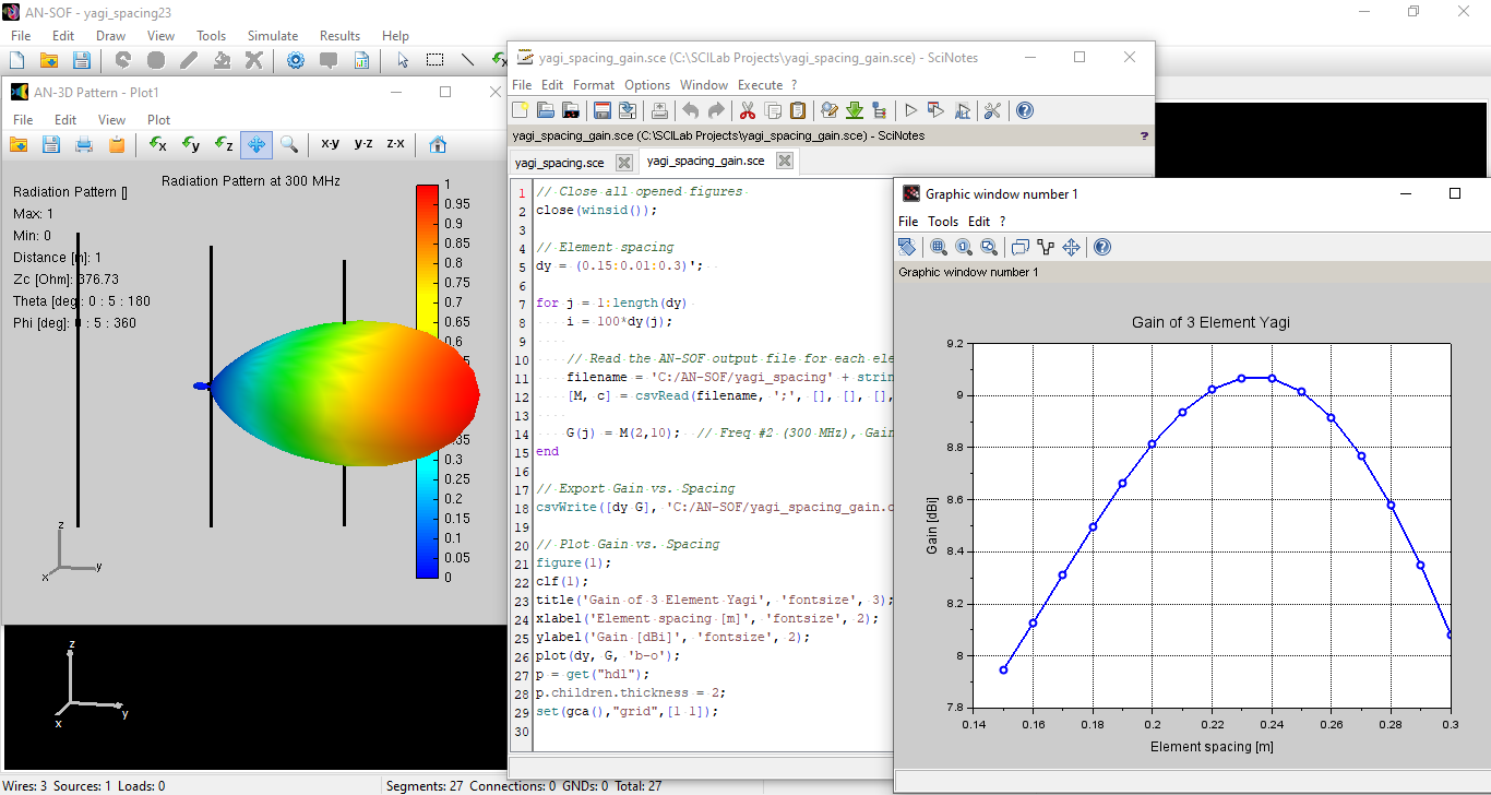
yagi_spacing_gain.sce

It reads each of the output files having the “PowerBudget” tag and extracts the gain at the frequency of 300 MHz. Pay attention to this line,

// Read the AN-SOF output file for each element spacing

    filename = 'C:/AN-SOF/yagi_spacing' + string(i) + '_PowerBudget.csv';

If you have chosen a directory other than C:/AN-SOF/, declare it by changing this line.

Also, pay attention to this line,

// Export Gain vs. Spacing

csvWrite([dy G], 'C:/AN-SOF/yagi_spacing_gain.csv');

This is the full path, with directory and filename, where the extracted gain versus element spacing data will be exported. This line is optional, you can comment it out by adding “//” at the beginning if you don’t want to export a file with the data. Now run this script and you will see a plot of gain versus element spacing.