Evaluating EMF Compliance – Part 2: Using Near-Field Calculations to Determine Exclusion Zones

In this article, we dive deep into near-field calculations to establish RF exclusion zones. By understanding near-field and far-field regions, occupational vs. public exposure, health impacts, and practical methods, we ensure compliance with EMF guidelines and safeguard human health.

Key Takeaways:

• Near-field calculations are crucial: Understanding and applying near-field calculations help establish accurate RF exclusion zones, ensuring compliance and safety.

• Different exposure limits: Differentiating between occupational and public exposure is key due to varying health statuses and training levels.

• Practical applications: Using methods like the concentric sphere approach aids in determining compliance boundaries effectively.

• Continuous updates: Staying informed about evolving EMF guidelines and regulations is essential for maintaining safe RF transmission practices.

Introduction

In the first part of this two-article series, we discussed the guidelines published by the International Commission on Non-Ionizing Radiation Protection (ICNIRP), which outline safety thresholds or reference levels for exposure to radio frequency (RF) electromagnetic fields (EMF) in the frequency range of 100 kHz to 300 GHz. The ICNIRP 1998 guidelines were adopted by regulatory authorities in many countries, with most now updating their regulations to the new ICNIRP 2020 guidelines.

In part 1, we highlighted differences between regulations in various countries, using the US (FCC rules) and UK (Ofcom rules) as examples. We noted that, in the far-field region of antennas, the Effective Isotropic Radiated Power (EIRP) can be used as a metric when assessing the RF compliance of radio transmitting stations. Both the FCC and Ofcom have criteria to determine when a station is exempt from performing an assessment. We demonstrated, using a delta loop beam array antenna for the 17m band, that these criteria yield different results; the same equipment configuration may be exempt in the US but not in the UK. This underscores the importance of being aware of the RF limits set by the country or region where we are transmitting.

This part 2 article explains how to establish an exclusion zone around an antenna based on near-field calculations. This method complements far-field calculations using the EIRP, which often provide conservative values. Nevertheless, being conservative with EMF estimates is a good practice to ensure compliance with regulations and safety thresholds for human RF exposure.

Understanding Antenna Near-Field and Far-Field Regions

The criteria for determining when a station is exempt are based on calculations in the far-field region of antennas. The EIRP (Effective Isotropic Radiated Power) is a metric that is well-defined only in this region, where it remains independent of the distance to the antenna. Therefore, it is crucial to establish the boundary between the near-field and far-field regions to effectively use the EIRP. Since the EMF (electromagnetic field) radiated from an antenna decreases with distance, following the inverse square law for power density in free space and in the far-field zone, the EIRP is used. The EIRP is obtained by multiplying the power density by the square of the distance, making it independent of the distance to the antenna. However, the definition of EIRP is only meaningful in the far-field region of antennas. In part 1 of this article, we reviewed the standard criteria used to determine the boundary between near-field and far-field regions, and a calculator based on these textbook criteria can be found here.

In the near-field region, the EMF can be extremely strong, even if the EIRP is relatively low in the far-field region. For this reason, the ICNIRP guidelines do not mention EIRP but instead reference levels for electric field strength (E, measured in Volts per meter [V/m]), magnetic field strength (H, measured in Amperes per meter [A/m]), and power density (S, measured in Watts per square meter [W/m²]). All these values are rms (root mean square), which are the practical values measured. Remember that rms values are “time averages” obtained by averaging the square of the quantity of interest over time and then taking the square root of the result. Root mean square values are the actual observable quantities obtained by measurement instruments. In part 1 of this article, we also discussed and emphasized the importance of time averages in performing EMF compliance calculations.

Having established this, it is clear that calculations based solely on EIRP and far-field equations do not provide information about field intensities in the near-field region. Although the FCC has published a table to calculate compliance distances for different frequency ranges and Ofcom sets a maximum of 100 W for EIRP for stations exempt from an assessment, it is important to note that all these calculations are based on far-field equations. Given the complexity of performing an assessment in the near-field zone, this approach prioritizes practicality over accuracy. The ARRL (American Radio Relay League) and RSGB (Radio Society of Great Britain) have implemented this approach in online calculators (see ARRL calculator and RSGB calculator), which serve as a first approximation but oversimplify the problem. For instance, to account for a lossy ground plane, only one “average” reflection coefficient is used, so the conductivity and dielectric constant of the soil cannot be specified in the published calculators. Additionally, at least two reflection coefficients—one for vertical polarization and one for horizontal polarization—should be considered even in far-field region calculations.

For stations that do not meet the exemption criteria (FCC) or the low power compliance criteria (Ofcom), a more rigorous assessment is required. Electric field, magnetic field, and power density must be calculated using near-field formulas to establish more precise exclusion zones. These near-field values are then compared with the established maximum reference levels to determine whether the station is EMF compliant. Near-field closed-form mathematical expressions are often highly complex and are only available for elementary or simple canonical antennas, such as electrically short dipoles or small loops. The complexity of the equipment configuration, involving antenna geometry, ground plane parameters, as well as power losses in the feeder and tuner, necessitates the use of antenna simulation software like AN-SOF to model all these intricacies.

Therefore, the assessment of RF exposure from amateur radio stations involves various considerations, including power thresholds, time averages, near-field, and far-field calculations. Understanding these factors is crucial for ensuring the safe operation of amateur radio equipment and minimizing potential health risks.

Differentiating Occupational and General Public Exposure

The ICNIRP guidelines differentiate between occupationally exposed individuals and members of the general public. Occupationally exposed individuals are adults exposed under controlled conditions associated with their job duties. They are trained to be aware of potential RF EMF risks and to employ appropriate harm-mitigation measures, and possess the sensory and behavioral capacity for such awareness and response. An occupationally exposed worker must also be part of an appropriate health and safety program that provides this information and protection.

The general public includes individuals of all ages and varying health statuses, including vulnerable groups or individuals who may have no knowledge of or control over their EMF exposure. These differences necessitate more stringent restrictions for the general public, as they may not be trained to mitigate harm or may lack the capacity to do so. Occupationally exposed individuals are not considered to be at greater risk than the general public, provided that appropriate screening and training account for all known risks. It is important to note that a fetus is defined as a member of the general public, regardless of the exposure scenario, and is subject to general public restrictions. Therefore, occupational/controlled and general public/uncontrolled reference levels are not the same.

Health Effects and Near-Field Quantities

Exposure to RF EMFs can cause nerve stimulation, as described in the ICNIRP 2010 guidelines, for frequencies up to 10 MHz due to induced electric fields within the body. The effect of this stimulation varies with frequency, typically described as a “tingling” sensation around 100 kHz. As frequency increases, heating effects predominate, and the likelihood of nerve stimulation decreases.

In addition to nerve stimulation, radiofrequency EMFs can affect the body through two primary biological effects: changes in membrane permeability and temperature rise. When low-frequency EMFs are pulsed, the power is distributed across a range of frequencies, including radiofrequency EMFs. If the pulse is sufficiently intense and brief, it may cause cell membranes to become permeable. The ICNIRP 2010 guidelines’ restrictions on nerve stimulation ensure that these permeability changes do not occur, so additional protection from the resultant RF EMFs is unnecessary. Membrane permeability changes have also been observed with 18 GHz continuous wave exposure. This effect requires very high exposure levels, far exceeding those needed to cause thermal harm. Thus, there is no need for specific restrictions against this effect, as those designed to protect against smaller temperature rises will suffice.

Radiofrequency EMFs can generate heat in the body, and it is crucial to keep this heat at safe levels. Extensive evidence indicates that the heat generated at very low exposure levels, such as within the ICNIRP 1998 basic restrictions, is not sufficient to cause harm. However, there is limited research on exposure levels above these basic restrictions. When there is a reasonable expectation of health impairment at lower temperatures than those shown to impair health via RF EMF exposure, ICNIRP uses these lower temperatures as a basis for its restrictions. For frequencies above 10 MHz, the main effect of electromagnetic waves is to heat biological tissues by exciting molecules, increasing temperature. Unlike ionizing radiation, such as X-rays, which can cause electrons to jump to higher energy levels, potentially damaging DNA, RF EMFs primarily cause thermal effects.

One figure used to evaluate the heating of tissues is the Specific Absorption Rate (SAR), which measures the rate at which RF energy is absorbed per unit mass of tissue (access to a SAR calculator). Based on SAR studies of canonical antennas operating in close proximity to the human body and numerical models of these antennas, regulatory authorities set maximum reference limits for the electric field, magnetic field, and power density to reduce exposure to RF EMFs. As the quantities used to specify basic restrictions can be difficult to measure, more easily evaluated quantities are also specified as reference levels. The reference level quantities relevant to the ICNIRP guidelines include incident electric field strength (E_inc in V/m) and incident magnetic field strength (H_inc in A/m), incident power density (S_inc in W/m²), plane wave equivalent incident power density (S_eq in W/m²), incident energy density (U_inc in J/m²), and plane-wave equivalent incident energy density (U_eq in J/m₂), all measured outside the body, and electric current inside the body (in Amperes).

With respect to the evaluation of EMF compliance, the metrics directly accessible for measurements outside the human body are those produced by the fields radiated by the antennas: the electric field vector ($\mathbf{E}$), the magnetic field vector ($\mathbf{H}$), and the power density vector ($\mathbf{S}$). Since we work in the frequency domain and with rms values, the components of these fields are complex numbers. The rms power density, in magnitude, is given by:

$\displaystyle S = | \mathbf{E} \times \mathbf{H}^*| \qquad (1)$

This general definition applies to any region of space, both near and far-field regions. In the far-field region, the fields behave as a transverse electromagnetic (TEM) plane wave, and the incident power density can be calculated as:

$\displaystyle S = \frac{|\mathbf{E}|^2}{Z_0} = Z_0 \, |\mathbf{H}|^2 \qquad (2)$

where $Z_0$ is the characteristic impedance of free space, approximately 377 Ohms (often also approximated as 120π Ohms). Equation (2) is also used to evaluate the plane wave equivalent incident power density ($S_{eq}$). It is important to emphasize that this equation is only valid for TEM plane waves in free space. In the far-field region, the wavefront is spherical, and the propagating wave is TEM, so equation (2) can be used in this zone since a sufficiently small portion of the wavefront can be approximated by a plane. Essentially, in the far-field region, an observer receives a practically TEM plane wave.

Sometimes, equation (2) is applied in the near-field region of antennas, but this is incorrect since the wave is not TEM or plane in this region. Instead, equation (1) should be used. In general, equation (1) gives the correct rms value of the power density in any region of space outside the surface of an antenna.

Starting with version 9.50, AN-SOF calculates the rms power density according to equation (1) automatically after running the calculation of the near E and H fields.

Limits for Maximum Permissible Exposure and Time Averages

Since the publication of the new ICNIRP guidelines in March 2020, some countries have updated their regulations to align with the new reference levels, while others have not. Therefore, it is crucial to determine the reference levels in the specific country or region where we are operating.

For instance, as of the latest information available, FCC OET Bulletin 65 Edition 97-01 is currently under review to incorporate updates related to recent rule changes. Although no official update to the bulletin has been released yet, a revised version is expected to reflect the new guidelines. Table 1 shows the limits for Maximum Permissible Exposure (MPE) for controlled and uncontrolled exposure according to the FCC bulletin 65b.

Exposure Scenario	Frequency Range (MHz)	E-Field Strength (V/m)	H-Field Strength (A/m)	Power Density S (W/m2)	Averaging Time |E|2, |H|2 or S (minutes)
Occupational	0.3 – 3.0	614	1.63	(1000)*	6
	3.0 – 30	1842/f	4.89/f	(9000/f2)*	6
	30 – 300	61.4	0.163	10.0	6
	300 – 1500	—	—	f/30	6
	1500 – 100,000	—	—	50	6
General Public	0.3 – 1.34	614	1.63	(1000)*	30
	1.34 – 30	824/f	2.19/f	(1800/f2)*	30
	30 – 300	27.5	0.073	2.0	30
	300 – 1500	—	—	f/150	30
	1500 – 100,000	—	—	10.0	30

In the first two rows, the power density is calculated using equation (2), representing the plane wave equivalent power density. In these cases, the magnetic field is given by H = E/Z₀, so it is sufficient to calculate the electric field intensity. For frequency ranges above 30 MHz, it is necessary to calculate the E and H fields separately and determine the power density using equation (1). The table also indicates that for frequencies above 300 MHz, only reference levels for power density are provided.

In the last column of Table 1, the averaging time is given in minutes. In terms of power density or rms values of E and H, the fields must be averaged over specific periods, ensuring the average does not exceed the limit for continuous exposure. As shown in Table 1, the averaging time for occupational/controlled exposures is 6 minutes, while for general public/uncontrolled exposures it is 30 minutes. It is important to note that for general public exposures, it is usually not possible to control access or limit exposure duration to the extent that averaging times can be applied. In these situations, continuous exposure to RF fields, created by the on/off cycles of the radiating source, should be assumed.

As an illustration of time-averaging application to occupational exposure at an amateur station, consider the following: the relevant interval for time-averaging for occupational exposures is 6 minutes. This means that during any given 6-minute period, an amateur or worker could be exposed to twice the applicable power density limit for 3 minutes, provided they are not exposed at all for the preceding or following 3 minutes. Similarly, a worker could be exposed to three times the limit for 2 minutes, as long as no exposure occurs during the preceding or subsequent 4 minutes, and so forth.

The concept of power averaging includes both on and off times, as well as the duty cycle (also known as duty factor) of the transmitting mode being used. Various modes of operation have their own duty cycles, representing the ratio between average and peak power. Table 3 in Part 1 of this article shows the mode factors (multiplicative factor) and the corresponding duty cycles (as percentages) for several modes. To calculate the average power, multiply the transmitter peak envelope power (PEP) by the mode factor, then multiply the result by the worst-case percentage of time the station would be on the air in a 6-minute period (for controlled exposure) or a 30-minute period (for uncontrolled exposure). In AN-SOF, we just need to choose the transmitting mode and the percentage of time transmitting, and the corresponding factors will automatically apply to the PEP, so manual calculations are unnecessary.

Regarding Ofcom in the UK, they have an online calculator with reference levels still based on the ICNIRP 1998 Guidelines. On their website, Ofcom has reproduced a table where the limits for the magnetic field and power density are calculated under plane wave assumptions, shown in Table 2 below.

Frequency Range Index	Min Frequency (MHz)	Max Frequency (MHz)	E-Field Strength (V/m)	H-Field Strength (A/m)	Power density S (W/m2)
0	1	10	61.518	0.365	—
1	10	400	28.000	0.073	2.000
2	400	2,000	1.945	0.005	0.009
3	2,000	300,000	61.000	0.160	10.000

The limitations of the Ofcom calculator are clarified in their technical notes and reproduced here:

The calculator in its current form has the following limitations:

• Only the reference levels for power density “S” are used to determine the compliance distance. In the far-field, the electric field strength “E”, the magnetic field strength “H” and “S” have a fixed relationship, i.e. E/H ≈ 377 ohms (the impedance of free space) and S = E × H. In the radiative near-field, the relationship between “E” and “H” is not strictly fixed but remains a reasonable approximation.
• Strictly speaking, the calculator is applicable to electromagnetically ‘short’ antennas (i.e. where the largest dimension, or the diameter of the antenna, is no greater than half the wavelength of its operating frequency). More advanced tools may need to be used for electromagnetically ‘long’ antennas (i.e. where the largest dimension, or the diameter of the antenna, is longer than half the wavelength of its operating frequency).
• As a conservative tool, the calculator does not take into account of the antenna characteristics or site geometry.
• The calculator will produce very conservative results if used to assess multiple transmitters in the way described in the ‘Guidance on Multiple Transmitters’ page. If the spectrum user cannot comply using this approach, we would suggest using alternative methods, e.g. using dedicated tools designed to handle multiple transmitters, carrying out measurements, etc.
• Using the calculator for surfaces with a high reflection coefficient (e.g. sea water, metal surfaces) may result in an underestimate of the compliance distance. Again, more advanced tools may be needed to obtain accurate results in such a scenario.

To mention another country example, in Australia, the national RF safety standard, RPS S-1, is heavily based on the ICNIRP 2020 guidelines. In Australia, RF EMF assessments are typically conducted by calculations rather than measurements, which is the usual form of assessment for mobile base stations. The Australian Standard for RF exposure assessments, AS/NZS 2772.2, requires that uncertainty assessments be conducted for all assessments. This provides a common gauge for comparing the quality of measured and calculated assessments. AS/NZS 2772.2 also stipulates an uncertainty decision rule, which applies a penalty to the assessment level if the uncertainty of the assessment exceeds a certain threshold. Of course, RF calculations can also be inaccurate due to errors, but this also applies to measurements. Dr. Vitas Anderson, Associate Professor at Swinburne University of Technology in Melbourne, Australia, has recently developed an online guide for conducting RF uncertainty assessments, which can be explored here: RF Uncertainty Guide.

The reference levels published by the ICNIRP in the 2020 guidelines is reproduced in Tables 3 and 4 below, where time averaged limits are presented over 6 minutes in Table 3 and over 30 minutes in Table 4. In each table, in turn, values for occupational exposure and for the general public are distinguished. This marks a difference from FCC Table 1.

Exposure Scenario	Frequency Range	Incident E-Field Strength; Einc (V/m)	Incident H-Field Strength; Hinc (A/m)	Incident Power Density; Sinc (W/m2)
Occupational	0.1 – 30 MHz	1504/fM0.7	10.8/fM	NA
	>30 – 400 MHz	139	0.36	50
	>400 – 2000 MHz	10.58 fM0.43	0.0274 fM0.43	0.29 fM0.86
	>2 – 6 GHz	NA	NA	200
	>6 – <300 GHz	NA	NA	275/fG0.177
	300 GHz	NA	NA	100
General Public	0.1 – 30 MHz	671/fM0.7	4.9/fM	NA
	>30 – 400 MHz	62	0.163	10
	>400 – 2000 MHz	4.72 fM0.43	0.0123 fM0.43	0.058 fM0.86
	>2 – 6 GHz	NA	NA	40
	>6 – 300 GHz	NA	NA	55/fG0.177
	300 GHz	NA	NA	20

Notes for Table 3:

1. “NA” signifies “not applicable” and does not need to be taken into account when determining compliance.
2. f_M is frequency in MHz; f_G is frequency in GHz.
3. S_inc, E_inc, and H_inc are to be averaged over 6 min, and where spatial averaging is specified in ICNIRP 2020 Notes 6–7, over the relevant projected body space. Temporal and spatial averaging of each of E_inc and H_inc must be conducted by averaging over the relevant square values (see ICNIRP 2020 Appendix A for details).
4. For frequencies of 100 kHz to 30 MHz, regardless of the far-field/near-field zone distinctions, compliance is demonstrated if neither peak spatial Einc or peak spatial Hinc, over the projected whole body space, exceeds the above reference level values.
5. For frequencies of >30 MHz to 6 GHz: (a) within the far-field zone, compliance is demonstrated if one of peak spatial S_inc, E_inc or H_inc, over the projected whole-body space, does not exceed the above reference level values (only one is required); S_eq may be substituted for S_inc; (b) within the radiative near-field zone, compliance is demonstrated if either peak spatial S_inc, or both peak spatial E_inc and H_inc, over the projected whole-body space, does not exceed the above reference level values; and (c) within the reactive near-field zone: compliance is demonstrated if both E_inc and H_inc do not exceed the above reference level values; S_inc cannot be used to demonstrate compliance; for frequencies >2 GHz,
   reference levels cannot be used to determine compliance, and so basic restrictions must be assessed.
6. For frequencies of >6 GHz to 300 GHz: (a) within the far-field zone, compliance is demonstrated if S_inc, averaged over a square 4-cm² projected body surface space, does not exceed the above reference level values; S_eq may be substituted for S_inc; (b) within the radiative near-field zone, compliance is demonstrated if S_inc, averaged over a square 4-cm² projected body surface space, does not exceed the above reference level values; and (c) within the reactive near-field zone reference levels cannot be used to determine compliance, and so basic restrictions must be assessed.
7. For frequencies of >30 GHz to 300 GHz, exposure averaged over a square 1-cm² projected body surface space must not exceed twice that of the square 4-cm² restrictions.

Exposure Scenario	Frequency Range	Incident E-Field Strength; Einc (V/m)	Incident H-Field Strength; Hinc (A/m)	Incident Power Density; Sinc (W/m2)
Occupational	0.1 – 30 MHz	660/fM0.7	4.9/fM	NA
	>30 – 400 MHz	61	0.16	10
	>400 – 2000 MHz	3 fM0.5	0.008 fM0.5	fM/40
	>2 – 300 GHz	NA	NA	50
General Public	0.1 – 30 MHz	300/fM0.7	2.2/fM	NA
	>30 – 400 MHz	27.7	0.073	2
	>400 – 2000 MHz	1.375 fM0.5	0.0037 fM0.5	fM/200
	>2 – 300 GHz	NA	NA	10

Notes for Table 4:

1. “NA” signifies “not applicable” and does not need to be taken into account when determining compliance.
2. f_M is frequency in MHz.
3. S_inc, E_inc, and H_inc are to be averaged over 30 min, over the whole-body space. Temporal and spatial averaging of each of E_inc and H_inc must be conducted by averaging over the relevant square values (see ICNIRP 2020 Appendix A for details).
4. For frequencies of 100 kHz to 30 MHz, regardless of the far-field/near-field zone distinctions, compliance is demonstrated if neither E_inc or H_inc exceeds the above reference level values.
5. For frequencies of >30 MHz to 2 GHz: (a) within the far-field zone: compliance is demonstrated if either S_inc, E_inc or H_inc, does not exceed the above reference level values (only one is required); S_eq may be substituted for S_inc; (b) within the radiative near-field zone, compliance is demonstrated if either S_inc, or both E_inc and H_inc, does not exceed the above reference level values; and (c) within the reactive near-field zone: compliance is demonstrated if both E_inc and H_inc do not exceed the above reference level values; S_inc cannot be used to demonstrate compliance, and so basic restrictions must be assessed.
6. For frequencies of >2 GHz to 300 GHz: (a) within the far-field zone: compliance is demonstrated if S_inc does not exceed the above reference level values; S_eq may be substituted for S_inc; (b) within the radiative near-field zone, compliance is demonstrated if S_inc does not exceed the above reference level values; and (c) within the reactive near-field zone, reference levels cannot be used to determine compliance, and so basic restrictions must be assessed.

Taking the ICNIRP guidelines as a beacon, we could say that Table 1 (FCC) presents more up-to-date reference levels than Table 2 (Ofcom). Radiofrequency basic restrictions and reference levels are based on the lowest RF exposure levels that may cause adverse health effects. Since these health effects are related to temperature rises caused by exposure, they are determined by the energy or power of the RF exposure. Consequently, squared values of E and H are considered for time or spatial averages, or where multiple frequencies are summed.

Insights on Spatial Averages

The ICNIRP 2020 guidelines discuss spatial averages and averages over the whole-body space. Space averaging becomes important when the size of a person is comparable to the wavelength, especially in the near-field region of antennas. While a detailed discussion of spatial averages is beyond the scope of this article, it is important to understand that if the field distribution in the area of interest (such as a human body) is not uniform, it is not enough to measure the EMFs at a single point. Instead, fields should be measured at several points, averaging the square of the E and H fields and then taking the square root of the result.

However, if the area of interest is small compared to the wavelength, field variations may be negligible, and spatial averaging can be avoided. For example, if we are operating in the 20m band (14.000 MHz to 14.350 MHz), the average person is less than 10% of the wavelength’s size. Thus, we could avoid calculating space averages when operating in this band or at lower frequencies. Nevertheless, near fields in the reactive zone do not necessarily follow this rule, so it is crucial to evaluate the field distribution in the area of interest to determine if spatial averages are necessary.

For those interested in exploring spatial averages further, we highly recommend the resources at the Spatial Averaging Project, led by Dr. Vitas Anderson, along with a team from various companies and the Australian government. This project provides documentation and a data repository for developing a validated spatial averaging scheme for reference level limits on whole body ambient exposure to electric (E), magnetic (H), and power flux density (S) radiofrequency electromagnetic fields (RF EMF) in accordance with the new ICNIRP 2020 RF safety guidelines, the Australian ARPANSA RPS S-1 standard (based on ICNIRP), and the ICES IEEE 95.1:2019 standard.

Methods for Determining Compliance Boundaries or Exclusion Zones

Having a table with reference levels or limits for the maximum permissible exposure to RF, including values for the electric field, magnetic field, and power density across different frequency ranges, as established and approved by the regulatory authority of the country where we are operating, provides the necessary information to determine a compliance boundary around the antenna or transmitting station.

The exclusion zone is the region of space delineated by the maximum permissible limits of E, H, and S. Due to the complex near-field distribution, the exact exclusion zone generally does not have a regular shape; rather, it resembles an “amorphous bubble” around an antenna. To simplify and remain conservative, we will always consider the worst-case scenario. This means ensuring that E, H, and S are each below their respective maximum limits since we do not expect only one to meet the reference level.

According to Tables 1, 3, and 4, there will be an exclusion zone for occupational/controlled areas and another for the general public/uncontrolled areas. In the exclusion zone for the general public, measures must be taken to prevent people from circulating in those areas. If the exposure time is controllable, the average time spent must be considered, as the limits are time averages, as previously discussed. In some countries, it is recommended to place signage indicating the risk of RF exposure and to erect physical barriers, such as fences, to delimit the exclusion zone. When in doubt, the worst-case scenario should always be considered.

Given the complex spatial distribution of E, H, and S fields in the near-field region, determining an exclusion zone can be challenging. Therefore, devising a simple method for determining the exclusion zone is practically necessary, always considering the worst-case scenario.

Concentric Sphere Method

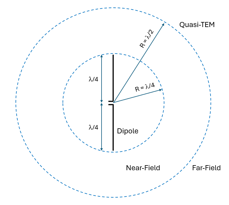
No matter how complex the near-field distribution is, there is always a distance far enough from the antenna where the wavefront begins to be spherical and the EMFs begin to behave as a TEM spherical wave. This distance is not necessarily very far from an antenna. For example, if we enclose a half-wave dipole within a quarter-wave radius sphere and then increase the sphere radius, at a half-wavelength from the dipole, we will notice a quasi-TEM wave, as illustrated in Figure 1. In the article Wave Matching Coefficient: Defining the Practical Near-Far Field Boundary, a coefficient called the “Wave Matching Coefficient (WMC)” is introduced. This coefficient helps determine the minimum sphere around the antenna that can be considered the boundary between the near and far field based on a margin of error measured in decibels.

Based on this idea, we will then consider concentric spheres of increasing radii over which we will calculate the rms values of the electric field (E), the magnetic field (H), and the power density (S). The sphere from which the values of E, H, and S do not exceed the reference values or maximum permissible exposure limits will determine the exclusion zone or compliance boundary.

This is the theory. In the real world, people walk on the ground. Therefore, if the antenna is elevated to a certain height, we should calculate the EMF in concentric rings with increasing radius from the projection of the antenna onto the ground.

The question arises of where to take the center for concentric spheres or rings. From the far-field point of view, the antenna reduces to a single point, making the center of the antenna less critical as we move away from it. Taking the antenna’s geometric center or the point where the feed point is located are reasonable options at first glance.

We will exemplify this method for the 17m Band 2-Element Delta Loop Beam discussed in part 1 of this article.

Delta Loop Beam Analysis in Free Space

The two-element delta loop beam design for the 17m band has been previously featured in this article: The 17m Band 2-Element Delta Loop Beam: A Compact, High-Gain Antenna for DX Enthusiasts. This antenna has a compact form factor, relatively large gain, and is virtually self-resonant with an input impedance close to 50 Ohms, eliminating the need for an impedance matching network. Because of these features, it is an ideal choice for DX enthusiasts.

In part 1 of this article, the VSWR in the range of 18.068 to 18.168 MHz was analyzed, as well as the radiation pattern and the EIRP. Here, we will focus on the near field of this antenna at the center frequency of 18.1 MHz.

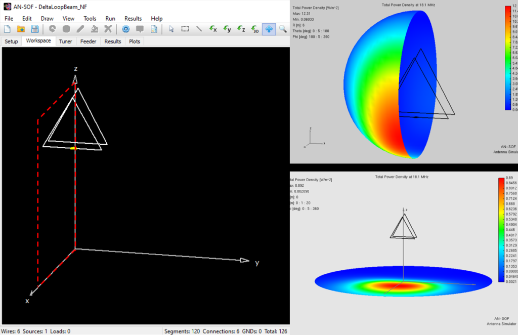
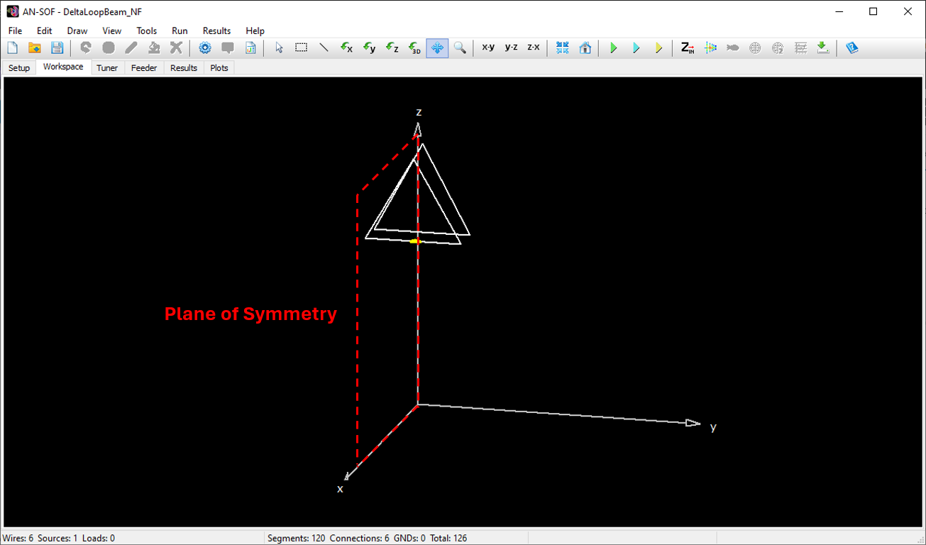
The geometric center of the antenna is located at the point (0, 0, 12.5m). Despite being in free space, a point elevated at 12.5m with respect to the XY plane (Z = 0) is chosen, as a ground plane at Z = 0 will be added later. Therefore, we will calculate the near field on a sphere centered at (0, 0, 12.5m). To enter the grid of points where the near field will be calculated, we must go to the Near-Field panel of the Setup tab. There, we will select the Spherical option (see Figure 2) since we are interested in calculating the E, H, and S fields on a sphere as explained. We can enter the origin (0, 0, 12.5m) (center of the sphere) and the range of variation of R (sphere radius), Theta (zenith angle), and Phi (azimuth angle). For a sphere to be complete, we enter the ranges 0 ≤ Theta ≤ 180 deg and 0 ≤ Phi ≤ 360 deg. However, this antenna has a plane of symmetry, which is the xz-plane according to the chosen orientation within the coordinate system (see Figure 3). Therefore, we will enter the angles varying in the ranges 0 ≤ Theta ≤ 180 deg and 180 ≤ Phi ≤ 360 deg, since it is only necessary to calculate the fields in a hemisphere.

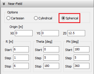
With regard to the range of variation of the radius “R” of the spheres, it is advisable to start with a radius just above the minimum radius of the sphere enclosing the antenna. Since each side of the triangular loop of each antenna element measures about 6m, we will choose an initial radius of 6m.

Figure 4 shows, from left to right, the E, H, and S fields on the 6m radius hemisphere. To generate these graphs, navigate to the main menu in AN-SOF > Results > Plot Near E-Field Pattern > 3D Plot to graph the E-field, and repeat the same steps for the H and S fields. The graphs in Figure 4 present a color scale where you can see the intensities, particularly the maximum intensity, which is the key value for comparison with the reference values or maximum permissible limits. Additionally, the charts display the maximum and minimum values in the legend at the top left of each chart.

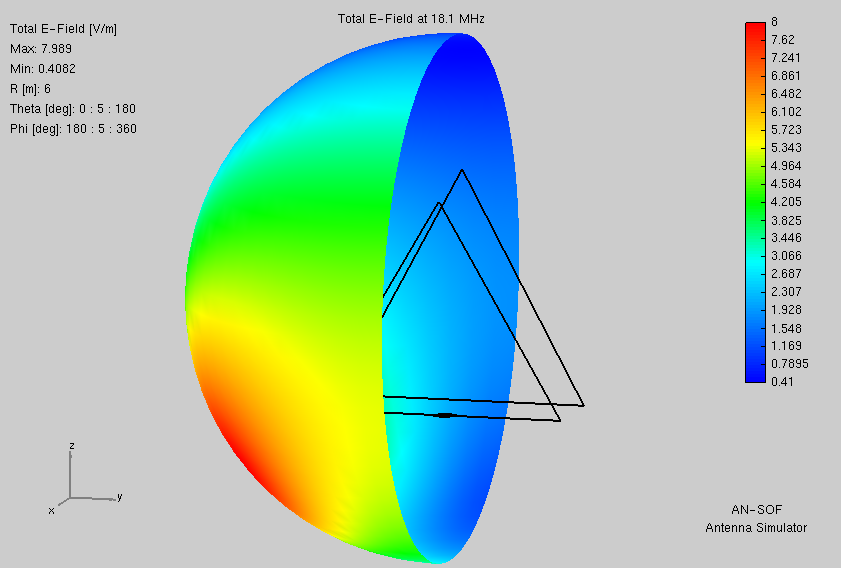
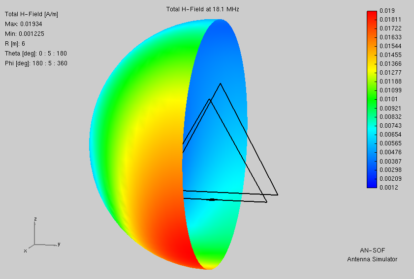
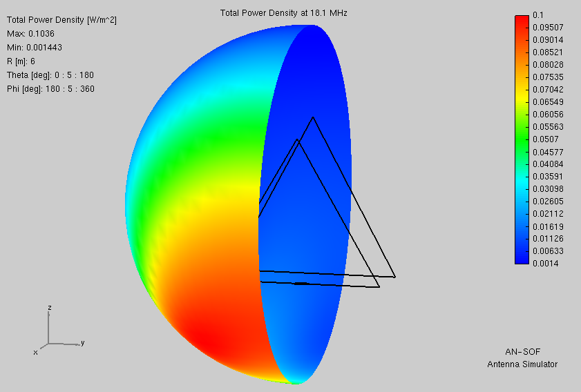
Fig. 4: E, H, and S fields on a sphere enclosing the antenna in the near-field region (free space).

In this example, the input power has been set to 10 W. We observe the maximum values of the fields are:

• E_max = 7.99 V/m

• H_max = 0.0193 A/m

• S_max = 0.104 W/m²

We will reference Table 1 of the FCC still in force in the US. For the frequency range of 3.0 – 30 MHz for controlled exposure, we get:

• E_ref = 1842/f = 1842/18.1 = 102 V/m

• H_ref = 4.89/f = 4.89/18.1 = 0.27 A/m

• S_ref = 1000 W/m²

Although we are very close to the antenna, with an input power of 10 W, we are well below the reference values. To reach the reference values, we would have to increase the power by more than 12 times. In these cases, regulatory authorities recommend establishing a minimum separation distance from the antenna, even if the safety limits have not been exceeded. The FCC recommends the near-field formula: R = λ/(2π) = 17m / (2π) = 2.7 m. Therefore, we would consider a radius of 2.7m from the geometric center of the antenna as an exclusion zone. In the UK, Ofcom stipulates that the safety distance must be at least 2.4m (8 ft).

In conclusion, we must verify if the values of E, H, and S exceed the maximum limits when feeding this antenna with more than 100 W. It should be clarified that a duty cycle below 100% will reduce the values of E, H, and S by the same percentage. Additionally, if we are not transmitting continuously for 6 or 30 minutes, the time-averaged power will be even lower, reducing the fields by the same fraction.

Delta Loop Beam Raised Above a Ground Plane

Adding a ground plane significantly affects EIRP values, as we have seen in part 1 of this article. However, regarding the near field, the previous section’s example of the antenna in free space indicates that we do not expect the values of E, H, and S to exceed the reference values at a 6m distance with an input power of 10 W. To illustrate, we will increase the power to 1,000 W. According to the original FCC rules, this power, for exceeding 500 W (see Table 1 in part 1), would require an evaluation, making our station non-exempt.

Let’s examine the results of the simulation in AN-SOF. Figure 5 shows the graphs of E, H, and S on a 6m radius hemisphere centered on the antenna, as in Figure 4.

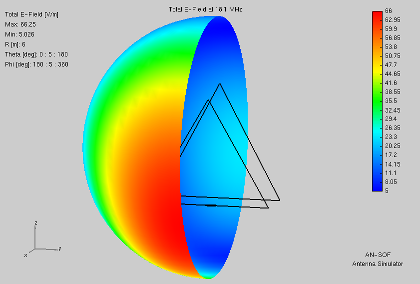
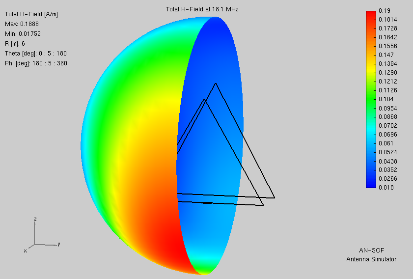
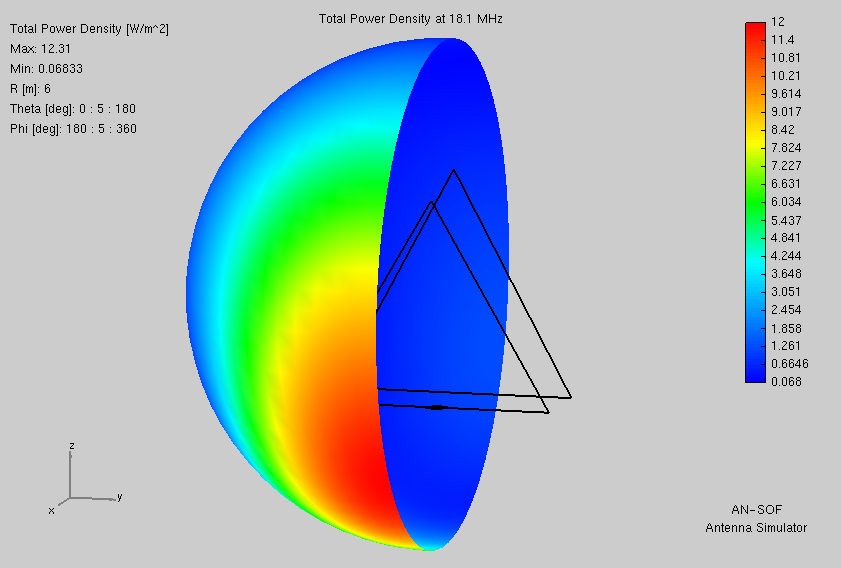
Fig. 5: E, H, and S fields on a sphere enclosing the antenna in the near-field region (above ground).

The maximum values obtained are:

• E_max = 66.3 V/m

• H_max = 0.189 A/m

• S_max = 12.3 W/m²

We see that even with 1,000 W of input power, we are below the reference values for maximum RF exposure.

In part 1 of this article, the effect of losses in the antenna feeder was also analyzed. When there are losses in the feeder, the power effectively delivered to the antenna terminals is reduced, and thus the values of E, H, and S will also be reduced.

To determine an exclusion zone at ground level, it is useful to plot the E, H, and S fields on the ground plane (plane Z = 0). In this case, instead of choosing spherical coordinates, we will choose cylindrical coordinates, as shown in Figure 6. Here, we will calculate the fields in concentric circles centered on the coordinate origin (0,0,0). We will vary the radius “R” of the circles from 0 to beyond a wavelength, up to 20m away. The results are shown in Figure 7.

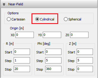
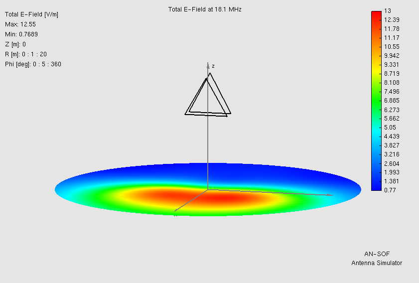
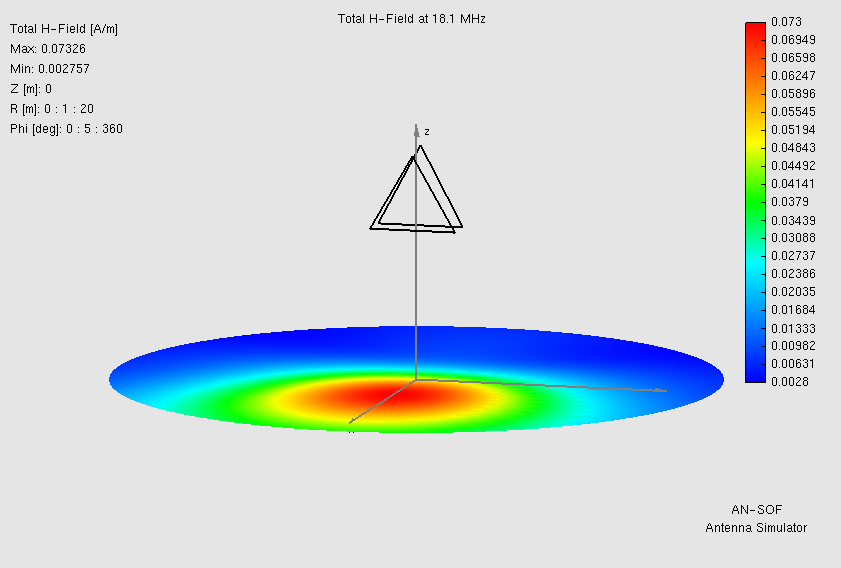
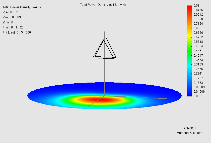
Fig. 7: E, H, and S fields at ground level below the antenna.

For this example, even at 1000 W, the values at ground level do not exceed the reference values. However, the graphs allow us to see how we could delimit an exclusion zone.

Conclusions

In this second part of our series on evaluating EMF compliance, we’ve delved into the nuances of near-field calculations and their crucial role in determining exclusion zones. By understanding the difference between near-field and far-field regions, and applying specific methods like the concentric sphere approach, we can better ensure that RF exposure remains within safe limits.

We highlighted the importance of differentiating between occupational and general public exposure, noting the stricter limits set for the general population due to their varied health statuses and lack of training in EMF safety measures. Additionally, we explored the health effects associated with RF EMF exposure, particularly focusing on nerve stimulation and heating effects, which underscore the necessity of rigorous compliance measures.

Our discussion on limits for maximum permissible exposure and time averages shed light on the significance of spatial and temporal averaging in assessing RF safety. We demonstrated practical applications of these principles through detailed analyses of the delta loop beam antenna, both in free space and when raised above a ground plane.

Overall, establishing clear compliance boundaries and exclusion zones based on near-field calculations not only helps in meeting regulatory requirements but also in safeguarding human health. As technology and guidelines evolve, staying informed and applying these principles will be essential for responsible and safe operation of RF transmitting equipment.

Disclaimer

Golden Engineering Ltd., developer of the AN-SOF Antenna Simulation Software, strives to provide accurate and reliable software for antenna modeling and simulation. However, the company assumes no responsibility for the consequences of using the software or the results obtained from its use. It is the sole responsibility of the software user or the person performing the calculations to ensure the accuracy and validity of the results. AN-SOF has been developed with the utmost diligence, incorporating numerical calculation methods aligned with the current state of the art in Computational Electromagnetics. Furthermore, the AN-SOF Knowledge Base provides numerous articles that validate the software’s calculations against theoretical and experimental results.

Despite these efforts, errors may occur due to user input, misinterpretations of results, or other factors beyond the control of Golden Engineering Ltd. These errors could lead to incorrect EIRP values or inaccurate electromagnetic field assessments, potentially exposing individuals to impermissible levels of RF signals. Therefore, Golden Engineering Ltd. explicitly disclaims any and all liability for any harm, injury, or damage resulting from the use of the AN-SOF Antenna Simulation Software or the interpretation of its results. The software user or the person performing the calculations assumes full responsibility for the accuracy and validity of the results and their implications for public safety.

---