Search for answers or browse our Knowledge Base.
Guides | Models | Validation | Book
Validating Numerical Methods: Transmission Line Theory and AN-SOF Modeling
Validate AN-SOF numerical results against classical transmission line theory in this detailed study of a wire-over-ground-plane system. By utilizing the short-circuit and open-circuit impedance technique, we demonstrate how simulated data correlates with standard characteristic impedance formulas. This article provides a step-by-step procedure for modeling lines in the AN-SOF workspace and highlights the engine’s precision in handling image theory and near-field interactions for numerical method validation.
Transmission Line Validation
A critical benchmark for any computational electromagnetics (CEM) solver is its ability to accurately replicate the results of classical transmission line theory. While the Method of Moments (MoM) is typically associated with complex 3D radiators, it can also be used to model the distributed parameters of two-wire lines. By comparing simulated data against standard analytical formulas for characteristic impedance, we can validate the precision of the solver’s near-field calculations and its handling of ground plane interactions.
In this study, we model a single-wire transmission line situated above a Perfect Electric Conductor (PEC) ground plane. According to image theory, the ground plane creates a virtual mirror image of the wire, effectively forming a two-wire transmission line system. Using this configuration, we will determine the characteristic impedance ($Z_0$) based on simulated input impedance data.
Simulation Configuration and Setup
The validation process begins with a specific setup in the AN-SOF environment to ensure the simulation remains within the valid range of transmission line theory.
Step 1: Environment and Frequency
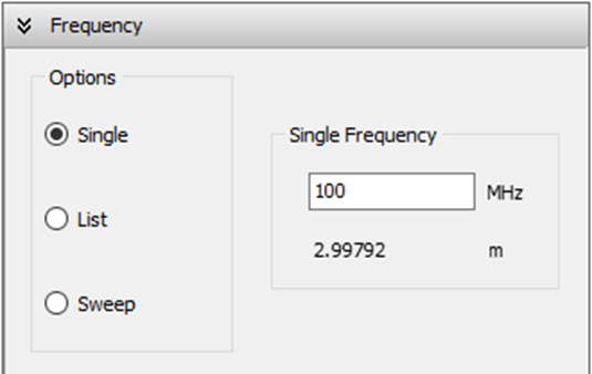
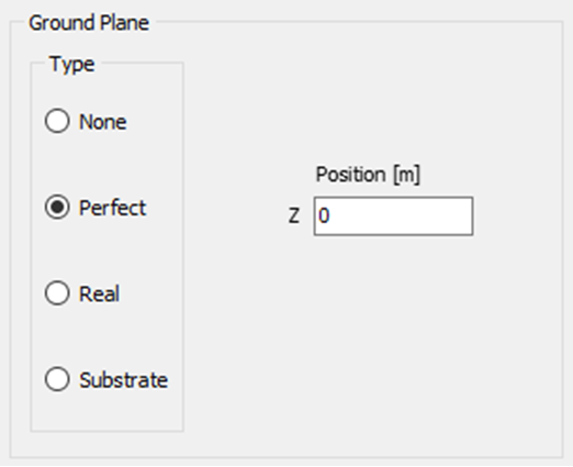
The frequency is set to $100 \text{ MHz}$ (as shown in Fig. 1a). It is vital to choose a frequency where the cross-sectional dimensions of the line are much smaller than the wavelength to ensure that the TEM (Transverse Electromagnetic) mode is dominant and higher-order modes are suppressed. The environment is configured with a perfect ground plane at $z = 0$ (Fig. 1b), which provides the necessary reflection for the return path.
Step 2: Geometry and Discretization
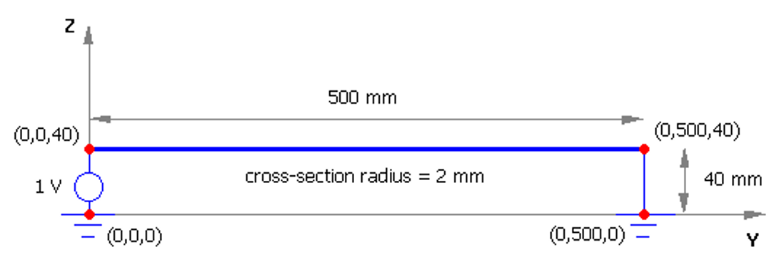
The transmission line is constructed using a single horizontal wire with the following dimensions:
- Length: $L = 500 \text{ mm}$.
- Height above ground: $h = 40 \text{ mm}$.
- Wire radius: $a = 2 \text{ mm}$.
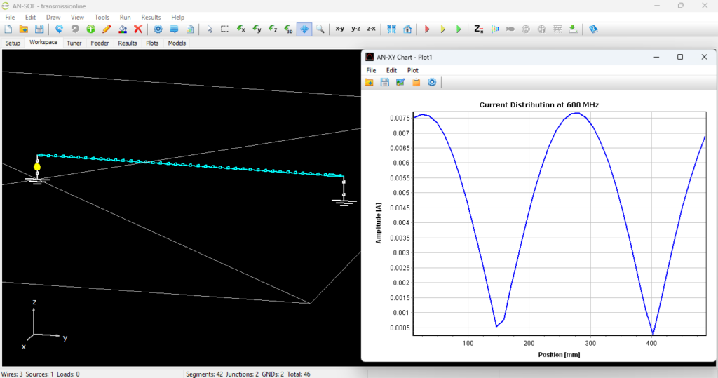
The horizontal wire is discretized into $40$ segments to ensure adequate current resolution. Two short vertical wires connect the ends of the transmission line to the ground. A voltage source is placed on the vertical wire at the start of the line (at coordinates $x = 0$, $y = 0$, $z = 40 \text{ mm}$) to excite the system, while the opposite end is short-circuited (Fig. 2).
Methodology: The Short-Circuit and Open-Circuit Technique
To determine the characteristic impedance ($Z_0$) of the line, we employ the classic relationship from transmission line theory, which states that $Z_0$ is the geometric mean of the input impedance when the line is short-circuited ($Z_{sc}$) and when it is open-circuited ($Z_{oc}$):
$\displaystyle Z_{0} \,=\, \sqrt{Z_{sc} \, Z_{oc}}$
The Short-Circuited Case:
Since a vertical wire is placed at the end of the line (at $y = 500 \text{ mm}$ in Fig. 2) to connect the horizontal wire to the ground plane, the line is short-circuited. Upon running the simulation, the input impedance is found to be primarily reactive and inductive. The result is:
- $Z_{sc} \approx +j 511\ \Omega$
While a small real part (approx. $1.6\ \Omega$) exists due to the radiation resistance of the structure, it is negligible for the purpose of $Z_0$ calculation.
The Open-Circuited Case:
The vertical wire short-circuiting the line is removed, leaving the end of the line floating; thus, the line is open-circuited. Rerunning the calculations provides the capacitive response of the line:
- $Z_{oc} \approx -j 105\ \Omega$
Comparative Analysis: Simulation vs. Theory
Using the values obtained from AN-SOF, the simulated characteristic impedance is calculated as:
$\displaystyle Z_{0} \,=\, \sqrt{511 \times 105} \,\approx\, 232\ \Omega$
To validate this result, we compare it to the theoretical expression for a wire of radius $a$ at a height $h$ above a PEC ground plane (assuming $h \gg a$):
$\displaystyle Z_{0} \,=\, 138 \, \log \left( \frac{2h}{a} \right)$
Substituting our values ($h = 40 \text{ mm}$, $a = 2 \text{ mm}$):
$\displaystyle Z_{0} \,=\, 138 \, \log \left( \frac{2 \times 40}{2} \right) \,\approx\, 221\ \Omega$
The agreement between the simulated $232\ \Omega$ and the theoretical $221\ \Omega$ is excellent. The small discrepancy (approximately 5%) is expected, as the theoretical formula is an approximation that assumes an infinitely long line and ignores the end effects and small radiation losses that the Method of Moments correctly includes.
Conclusion
This validation study demonstrates that AN-SOF accurately models the fundamental behavior of transmission lines through its explicit geometric representation. By successfully replicating the characteristic impedance predicted by classical theory, the simulation confirms that the engine’s near-field potential calculations and ground-plane mirror-image implementations are highly precise.
Furthermore, the study highlights that the Method of Moments provides a more comprehensive view than simple analytical formulas by accounting for the small but real radiation resistance present even in “guided” structures. For engineers and designers, this confirms that AN-SOF can be used not only for antenna design but also for modeling complex feed systems, matching networks, and interconnects where transmission line behavior is a critical factor in overall system performance.
See Also:
Technical Keywords: Transmission Line Theory, Characteristic Impedance, Image Theory, AN-SOF Validation, Numerical Methods, Short-Circuit Impedance, Open-Circuit Impedance, PEC Ground Plane, Method of Moments.
