Search for answers or browse our Knowledge Base.
Guides | Models | Validation | Book
A Simple, Low-Cost Approach to Simulating Solid Wheel Antennas at 2.4 GHz
Explore a simple, low-cost method to simulate 2.4 GHz solid wheel antennas with reliable first-order accuracy and practical efficiency.
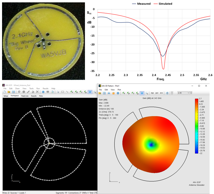
This article presents calculated return loss and gain results in the 2.4 GHz band for Wheel antennas. Using a simplified approach for simulating planar antennas on ungrounded dielectric substrates with sufficiently high permittivity, the results closely replicate the measured data published by the antenna manufacturer, achieving practical engineering accuracy. A summary of these results is shown in Figure 1. The proposed method is not only straightforward but also enables the use of cost-effective simulation tools.
Introduction
Wheel antennas derive their name from their circular configuration and the presence of spokes akin to a cartwheel. Among wheel antenna designs, solid wheel antennas feature flat metallic traces printed on a singular dielectric substrate. Typically, these substrates are circular and crafted from materials such as FR4. Solid wheel antennas are known for their compact dimensions and frequent application in ISM (industrial, scientific, and medical) frequency bands spanning from approximately 900 to 2400 MHz, primarily within wireless network contexts. In the plane of the wheel, these antennas offer omnidirectional coverage and exhibit horizontal polarization. Moreover, the radiation pattern in the plane perpendicular to the wheel closely resembles that of a magnetic dipole, taking on a distinctive donut-like shape.
This article centers on the examination of a 2.4 GHz wheel antenna manufactured by Kent Electronics (WA5VJB). Our primary objective is to replicate the measured return loss data (S11) for the Big Wheel Rev B antenna variant as provided by the manufacturer, available at this link.
Calculation Method
Given the planar nature of wheel antennas, fabricated on an ungrounded dielectric substrate, we can employ a straightforward method for simulating these microstrip antennas. This approach is outlined in the article Simplified Modeling of Microstrip Antennas on Ungrounded Dielectric Substrates: A Practical First-Order Approach, which offers a cost-effective means of modeling such antennas. This methodology capitalizes on the capabilities of wire antenna simulation software, such as AN-SOF.
The initial step involves defining the frequency range of interest, which, in this instance, spans from 2.2 to 2.6 GHz. Subsequently, the antenna structure is created within AN-SOF. This process is relatively uncomplicated and entails the addition of Line objects to represent the straight metallic strips and Arc objects to replicate the curved sections of the antenna. This wheel antenna boasts a diameter of approximately 1.5 inches. At the center of this circular structure, the feed point is positioned.
Radiating outward from the antenna’s center, there are spokes that connect to the arcs on the antenna’s periphery, situated above the dielectric substrate. Additionally, there are spokes that return beneath the substrate to close the electrical circuit of the antenna. For the sake of facilitating external connectivity, the manufacturer typically incorporates a coaxial connector at the antenna’s central point, enabling a straightforward connection to a coaxial cable.
AN-SOF, operating on the Conformal Method of Moments, mandates the division of wires into shorter segments relative to the wavelength. In the case of the antenna printed on FR4, which possesses a dielectric constant of 4.6, the applicable wavelength must be that of free space divided by √(4.6) = 2.14. Consequently, for the uppermost frequency within the specified range, 2.6 GHz, the wires have been partitioned into segments measuring 2% of the wavelength within the substrate. This aligns with the same criterion employed for planar dipoles, as detailed in the previously referenced article.
In accordance with the manufacturer’s datasheet, this antenna is tunable through the introduction of a capacitor with an approximate value of 1 pF. This tuning capacitor has been incorporated into the model at the feed point, inserted in series with a voltage source. By configuring a medium characterized by a permittivity of 4.6, as depicted in Figure 2, and initiating the calculations with a Ctrl + R command, we have ascertained that the antenna resonates at 2.43 GHz when equipped with a 0.7 pF capacitor, consistent with the datasheet’s specifications. Consequently, there is no necessity to determine the resonance frequency in free space, as elucidated in the simplified method. This instance exemplifies an alignment between the effective permittivity and the substrate’s permittivity.
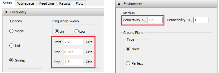
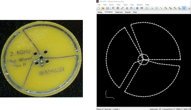
Figure 3, included below, presents a photograph of the physical wheel antenna, sourced from the manufacturer’s website, alongside the corresponding AN-SOF model, illustrating the employed segment density.
Comparison with Measured Data
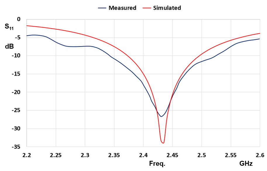
Initiating the input impedance calculation with a Ctrl + R command, within the scrutinized frequency span of 2.2 to 2.6 GHz and employing a medium permittivity of 4.6, we generate the S11 curve presented in Figure 4. This figure also overlays the measured S11 curve, extracted from the manufacturer’s datasheet. It is evident that the agreement between the simulated and measured outcomes is remarkably robust, particularly in the vicinity of the resonance frequency. It is worth noting that the model maintains good agreement with measurements, even though it completely neglects the dielectric substrate’s thickness and contour.
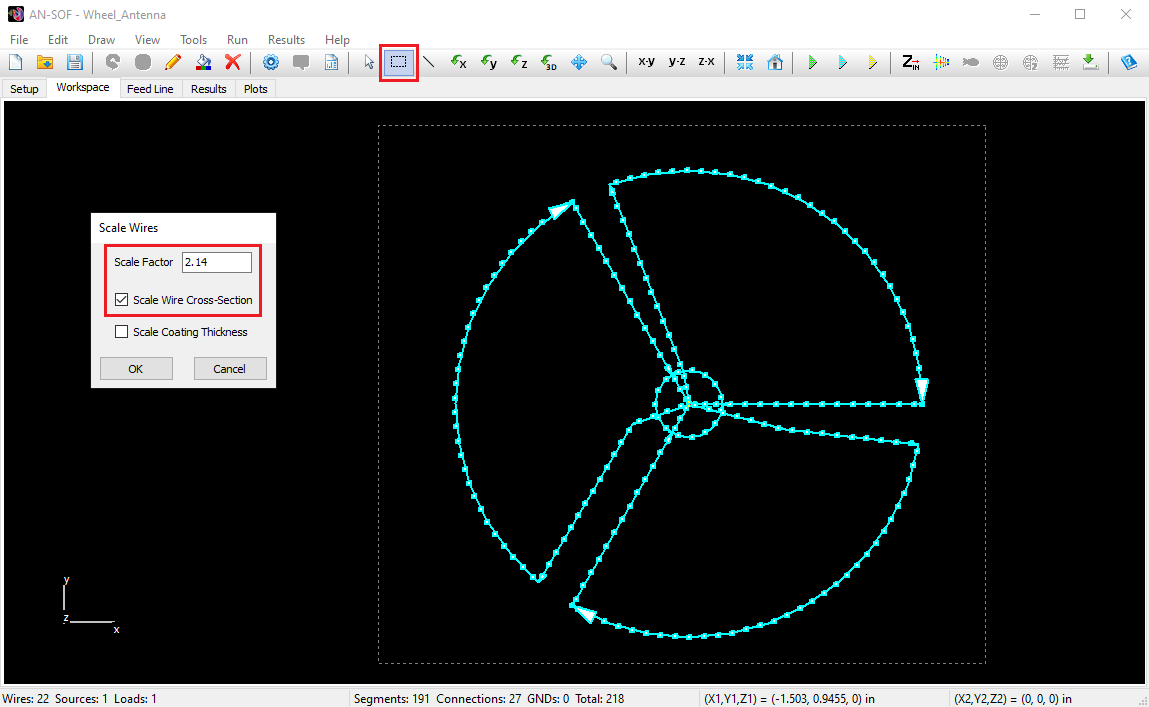
To calculate the radiation pattern, we must set the permittivity of the medium (free space) to 1, and then rescale the antenna’s dimensions by a factor of √(4.6) = 2.14. This can be achieved by first clicking on the “Selection Box” button within the AN-SOF toolbar. Subsequently, draw a box around the entire antenna using the mouse and then proceed to Edit > Scale Wires in the main menu. Here, input the scaling factor of 2.14, ensuring that you adjust the wire cross-section accordingly, as depicted in Figure 5. Furthermore, it is necessary to modify the value of the tuning capacitor, reducing it from 0.7 pF to 0.7/2.14 = 0.33 pF.
Once these adjustments are made, the calculation is tailored to the single frequency of 2.43 GHz, since our primary interest lies in the radiation pattern at the resonance frequency. With this configuration, we proceed with the calculations by pressing F11. The outcome, illustrated in Figure 6 (left), portrays the gain pattern in decibels (dBi), which, as anticipated, exhibits near-omnidirectional coverage within the plane of the antenna. Furthermore, the polarization is predominantly horizontal, evident from the dominance of the Eφ (azimuthal) component over the EΘ (zenithal) component of the electric field, as shown in Figure 6 (right). The Eφ component of the electric field reveals that there are three directions with radiation peaks, corresponding to each wheel arch, indicating that the radiation pattern is not perfectly omnidirectional.
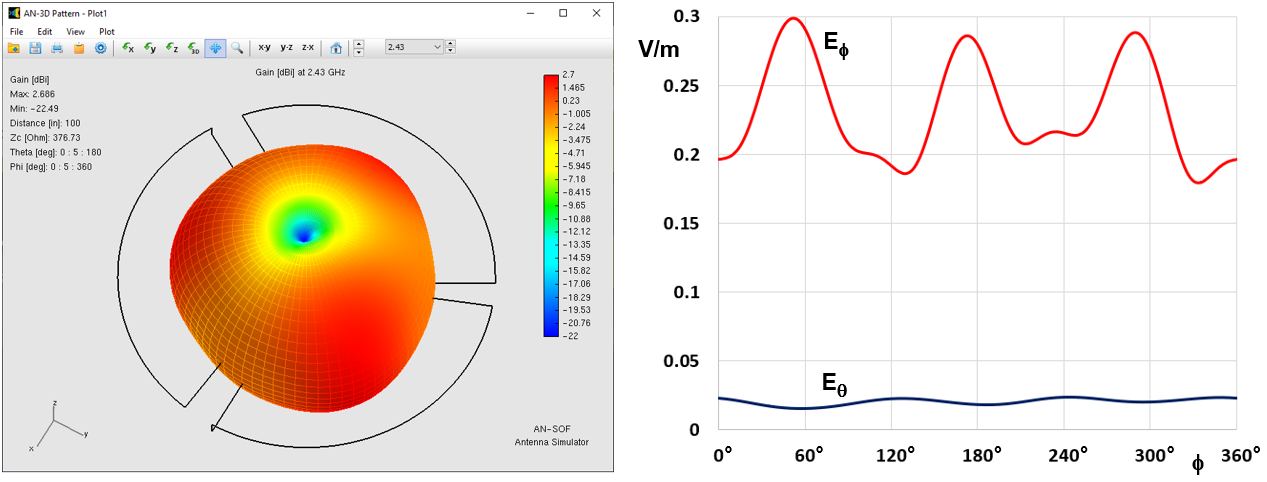
The calculated peak gain registers at 2.7 dBi, slightly surpassing the manufacturer’s specification of 2 dBi. It is essential to acknowledge that this computed gain does not account for all potential power losses within the actual antenna, particularly within components such as the coaxial connector and the substrate (incorporating loss tangent). These factors have been omitted in our model, wherein solely a resistivity matching that of aluminum has been introduced for the metal traces.
Conclusions
In this article, we have introduced a simplified method for the modeling of solid wheel antennas, enabling the calculation of their return loss and radiation pattern. We have employed this method to simulate the performance of the Big Wheel Rev B antenna designed for the 2.4 GHz band, as provided by Kent Electronics. The results obtained through AN-SOF simulation have been compared with the measured data furnished by the manufacturer, and a high degree of agreement has been achieved.
This study clearly demonstrates AN-SOF’s capability to model planar antennas printed on ungrounded dielectric substrates, such as FR4. The presented method combines simplicity with practical accuracy, making it a valuable tool for antenna engineers and researchers seeking cost-effective and reliable solutions for design and analysis.
