Defining the Environment

Environment and Ground Plane Options

The environment surrounding an antenna or metallic structure can be either free space or include a ground plane. In the case of free space, you can define the relative permittivity (dielectric constant ε_r) and magnetic permeability (µ_r) of the medium, with vacuum corresponding to ε_r = 1 and µ_r = 1.

Three ground plane options are available:

• Perfect Electric Conductor (PEC): An ideal, lossless ground plane.
• Real (Lossy) Ground: A ground plane with user-defined conductivity (σ) and relative permittivity (ε_r). Optionally, a radial ground screen can be added.
• Dielectric Substrate Slab: Used for modeling microstrip lines and printed antennas.

All ground planes lie in the xy-plane. The available environment settings will be described in detail in the sections below.

Configuring the Medium Properties

To configure the medium, navigate to the Setup tab > Environment panel. Use the Medium box (Fig. 1) to set the relative permittivity (ε_r) and permeability (µ_r) of the surrounding medium. When a ground plane is used, these values represent the permittivity and permeability of the medium above the ground.

Note:

The wavelength displayed below the frequency set in the Frequency panel (when the Single option is selected) and the wavelength used internally by AN-SOF for calculations will be adjusted based on the specified permittivity and permeability of the medium. Specifically, these properties cause the wavelength to shorten accordingly relative to the wavelength in a vacuum.

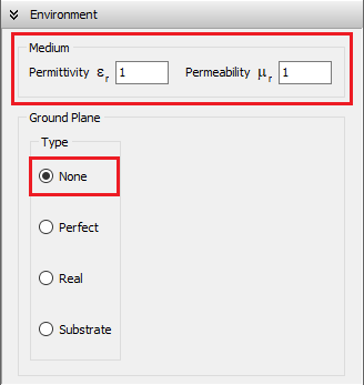
None (Free Space)

Selecting the None option simulates the antenna in free space. The relative permittivity (εᵣ) and permeability (µᵣ) specified in the Medium box (see Fig. 1) define the properties of the surrounding environment.

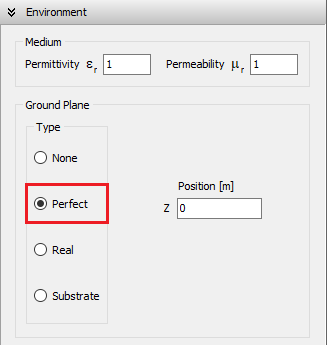
Perfect (PEC Ground)

Selecting the Perfect option places an infinitely large, perfectly electrically conducting (PEC) ground plane at a specified height relative to the xy-plane (see “Z Position” in Fig. 2). The ground plane remains parallel to the xy-plane, and its position is defined by the Z coordinate: a negative Z places the ground plane below the xy-plane, while a positive value places it above.

When using a perfect ground plane, all wires must be located above it—that is, each wire must have a Z-coordinate greater than or equal to the specified ground plane position. Wires crossing through or lying below the ground plane are not allowed. Additionally, horizontal wires placed directly on the ground plane are unsupported. However, connections from wire ends to the ground plane are permitted.

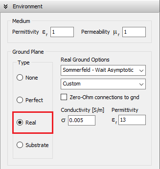
Real (Lossy Ground)

Selecting the Real option places a lossy ground plane at the xy-plane (z = 0), with user-defined conductivity (σ) and relative permittivity (εᵣ), as shown in Fig. 3. Four modeling methods are available for real ground calculations:

• Sommerfeld–Wait Asymptotic
• Reflection Coefficients
• Radial Wire Ground Screen
• Sommerfeld–Norton

These options are described in the following sections.

All wires must be positioned above the ground plane (z > 0). Horizontal wires directly on the ground plane are not supported.

Wire end connections to the ground are allowed when using either the Sommerfeld–Wait Asymptotic or Radial Wire Ground Screen options.

The Reflection Coefficients and Sommerfeld–Norton models assume perfect (zero-Ohm) wire connections to ground and yield reasonable results only for vertical wires connected to good conducting grounds—not dielectric surfaces. These models are not suitable when vertical wire-to-ground connections are made through dielectric materials.

Real Ground: Sommerfeld – Wait Asymptotic

This option models the antenna/wire currents using a hybrid approach that combines a perfect ground plane with loss impedances to account for power dissipation in the real ground—particularly important when wires are close to or connected to the ground. Developed by Prof. James R. Wait, this model is especially effective for low-frequency (LF) and medium-frequency (MF) antennas, where ground conductivity tends to be high. However, it remains applicable at higher frequencies as long as the ground behaves as a good conductor.

The model uses the ground’s conductivity (σ) and permittivity (εᵣ) to compute both near-field and far-field radiation, applying Norton’s asymptotic approximations to the exact Sommerfeld solution. The far-field results match those predicted by Fresnel reflection coefficients.

Wire connections to ground are supported. If a wire’s starting or ending point is located at z = 0, it will automatically be connected to the ground. These connections are treated as imperfect (lossy) by default, meaning power can be dissipated at the connection point due to current flow. If the Zero-Ohm connections to ground option is enabled, these connections are instead treated as perfect (lossless), though the presence of the lossy ground still influences the overall near and far fields.

In summary, the Sommerfeld – Wait Asymptotic model is appropriate when the ground can be considered a good conductor at the operating frequency and when the structure includes wire-to-ground connections.

Real Ground: Reflection Coefficients

When this option is selected, the ground conductivity (σ) and relative permittivity (εᵣ) influence the current distribution on the antenna or wire structure above the ground. As a result, the input impedance of a transmitting antenna is also affected by real ground conditions. This influence is determined using a generalization of Fresnel’s reflection coefficients, which is theoretically valid when wires are positioned several wavelengths above the ground. In practice, however, good results have been reported for heights between one-quarter and one-half of a wavelength.

Near fields are calculated using Norton’s asymptotic approximations to Sommerfeld’s exact solution, allowing the electric and magnetic fields to be computed as a function of distance from the antenna. This enables analysis of field attenuation due to ground losses. The far field, by contrast, is computed using the standard Fresnel reflection coefficients.

Vertical wire connections to ground may be added when the ground behaves as a good conductor at the operating frequency, even though these connections theoretically violate the height requirement. These wire-to-ground connections are treated as lossless in this model.

In summary, the Reflection Coefficients ground model is best suited for wire structures located several wavelengths above ground, ideally without any wire-to-ground connections. However, if the ground is a good conductor at the operating frequency, vertical wire connections may be included—but results under such conditions should be interpreted with caution.

Real Ground: Radial Wire Ground Screen

When this option is selected, a ground screen made of buried radial wires is placed on the ground plane, which has the specified conductivity (σ) and relative permittivity (εᵣ). The screen is centered at the origin (0,0,0), and its configuration is defined by user-specified parameters: the number of radial wires, their length (or screen radius), and wire radius. These wires are assumed to be laid on the ground surface or buried at a depth less than one soil skin depth.

This model is based on Prof. James R. Wait’s theory for good conducting grounds. It affects the current distribution on the antenna or wire structure by accounting for the power dissipated in the combined ground plane and wire screen system. As a result, both the presence of the screen and the ground properties (conductivity and permittivity) influence the input impedance of a transmitting antenna located above the screen. The same parameters are used to compute the radiated near and far fields using Norton’s asymptotic approximations to Sommerfeld’s solution and Fresnel reflection coefficients, respectively.

Wire-to-ground connections may be defined at wire endpoints located at z = 0. These are treated as imperfect by default, meaning that power is dissipated in the ground-screen system due to currents flowing between the ground and the wires. If the Zero-Ohm connections to ground option is enabled, these connections are treated as perfect, with no power dissipation at the contact point.

In summary, the Radial Wire Ground Screen model is suitable when the ground behaves as a good conductor at the operating frequency and when the structure includes wire-to-ground connections. The screen serves to increase the effective conductivity of the combined ground-screen system, reducing power losses beneath antennas placed above it. Typical use cases include monopole antennas in the form of poles or radiating towers used in broadcasting applications.

Real Ground: Sommerfeld – Norton

Unlike the previous ground models, which apply various approximations to compute the current distribution on wires above a lossy ground plane, the Sommerfeld–Norton model numerically solves Sommerfeld’s exact solution. This enables simulations where the ground does not need to be a good conductor—it may instead be a dielectric medium. To approximate a purely dielectric ground, enter a very low conductivity (e.g., σ = 1E-6 S/m) along with the desired relative permittivity (εᵣ).

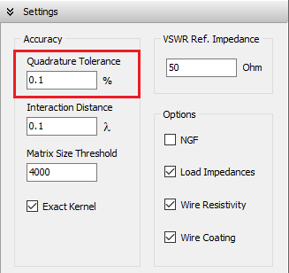
Vertical wires can be placed very close to the ground, with a minimum height of one wire radius above ground. Horizontal wires can be simulated as low as 0.005λ above ground. For vertical or horizontal wires at heights below 0.01λ, it is important to increase the accuracy of the calculations. To do this, go to Setup tab > Settings panel and set the Quadrature Tolerance to 0.1%, instead of the default 1% (see Fig. 4).

The near fields are computed from the current distribution using Norton’s asymptotic approximation to Sommerfeld’s solution. This is accurate at distances greater than about one-quarter wavelength from the wire structure, which is sufficient for most practical applications. The far field, in contrast, is calculated using Fresnel reflection coefficients, which yield the correct asymptotic expressions.

Wire-to-ground connections are theoretically not permitted in this model. However, they can be used with caution only for vertical wires, and only if the ground behaves as a good conductor at the operating frequency. In such cases, the model assumes lossless connections and employs specular reflection of the fields to compute the current distribution. These assumptions are valid only when the ground is effectively conductive.

In summary, the Sommerfeld–Norton model is the most accurate among the available ground models, but it comes with certain restrictions. It is recommended for highly dielectric grounds or situations where the ground cannot be considered a good conductor. Horizontal wires must not be placed below 0.005λ above ground. Vertical wires may be connected to ground only when the ground is a good conductor, and the results in such cases should be interpreted with care.

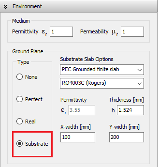
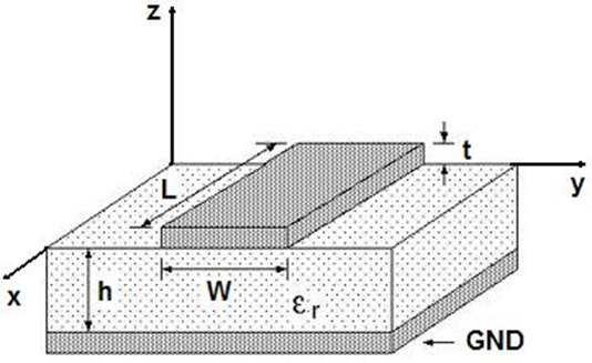
Substrate (Grounded Dielectric Slab)

When this option is selected, a dielectric substrate with user-defined relative permittivity (εᵣ) is placed beneath the xy-plane (z = 0), as shown in Figs. 5 and 6. The slab may extend infinitely or have finite dimensions in the xy-plane, where you can define its width along the X and Y directions. The substrate thickness, denoted as h, must also be specified. A perfectly electrically conducting (PEC) ground plane is located at z = –h, just below the dielectric slab (see Fig. 6). A drop-down list is available to select common substrate materials (e.g., FR4, RT/Duroid, Rogers RO). Note that the dielectric loss tangent cannot be specified—it is assumed to be zero, meaning the substrate is treated as lossless.

When the Substrate option is active:

• All wires must lie horizontally in the xy-plane (z = 0). These wires typically represent traces of printed antennas, microstrip lines, or PCB tracks.
• The only exception is for vertical wires (vias), which may connect traces at z = 0 to the ground plane at z = –h. These are commonly used to feed the structure with voltage or current sources.

Important constraints:

• The PEC ground plane beneath the substrate is mandatory and cannot be omitted. As a result, ungrounded dielectric substrates are not supported.
• Wires above the xy-plane (z > 0) or below the ground plane (z < –h) are not allowed in this model.

The Substrate model is an extension of the Conformal Method of Moments tailored for printed wire structures. It has the following limitations:

Model Limitations

Single-Layer, Lossless Substrate Only

• Only one dielectric layer is supported (multilayer stacks are not).
• The substrate must be lossless (loss tangent is assumed to be zero).
• No holes or cutouts are permitted in the substrate.

Finite-Size Substrate Constraints

• The substrate must be rectangular in shape.
• Traces must be placed at least 5× their width away from the substrate edges.

Ground Plane and Vias

• A PEC ground plane is always present and cannot be disabled.
• Vertical wires (vias) can be added to connect traces to the ground, typically for feeding.

No Slot-Based Designs

• Slot antennas or patches with slots cannot be modeled due to software limitations.