Search for answers or browse our Knowledge Base.
Guides | Models | Validation | Book
Validation of a Panel RBS Antenna with Dipole Radiators against IEC 62232 Standard
This article validates AN-SOF’s results against the IEC FDIS 62232 standard by replicating an RBS panel antenna model with nine dipole radiators. The successful validation highlights AN-SOF’s ability to deliver highly accurate results, even with relatively simple models.
Introduction
The IEC FDIS 62232 standard, published by the International Electrotechnical Commission (IEC), outlines methodologies for assessing radio-frequency (RF) field strength and specific absorption rate (SAR) in the vicinity of radiocommunication base stations (RBS). These measurements are critical for evaluating human exposure to RF emissions and ensuring compliance with safety regulations.
In this article, we validate the results obtained from AN-SOF, our antenna simulation software, by replicating a panel antenna model featuring nine dipole radiators. The model used for this validation is based on a reference design published by the IEC. An excerpt of the IEC document, which provides further details on the model, can be accessed via this link.
Modeling a Panel RBS Antenna with Dipole Radiators: Validation Setup in AN-SOF
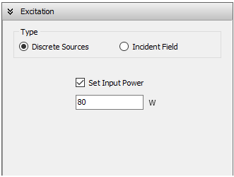
The RBS antenna under study comprises an array of nine vertical active dipoles, aligned and backed by a conductive panel reflector. Operating at 900 MHz, each dipole is individually excited by a source whose amplitude varies based on its position within the array. The total power delivered by the array is 80 W, calculated as the sum of the effective RMS power contributions from all nine sources. This total input power can be configured in AN-SOF via the Excitation panel under the Setup tab, as depicted in Figure 1.
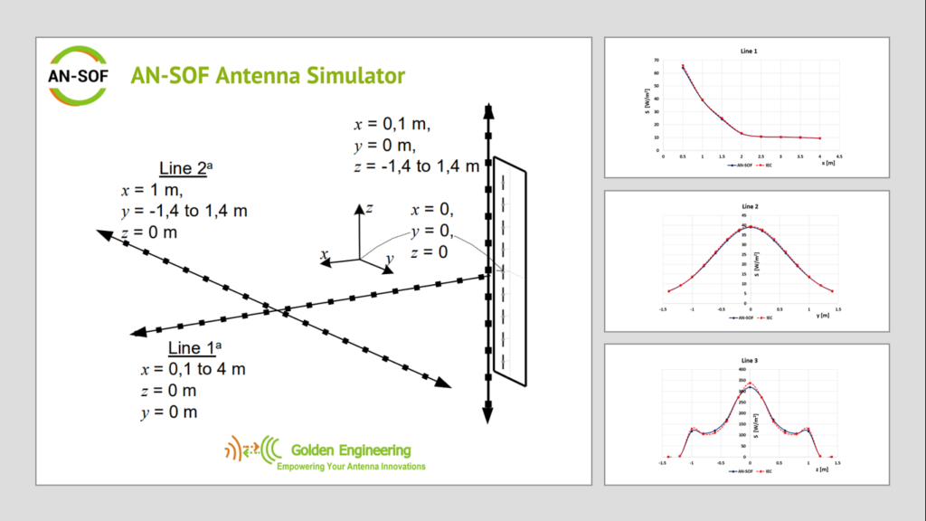
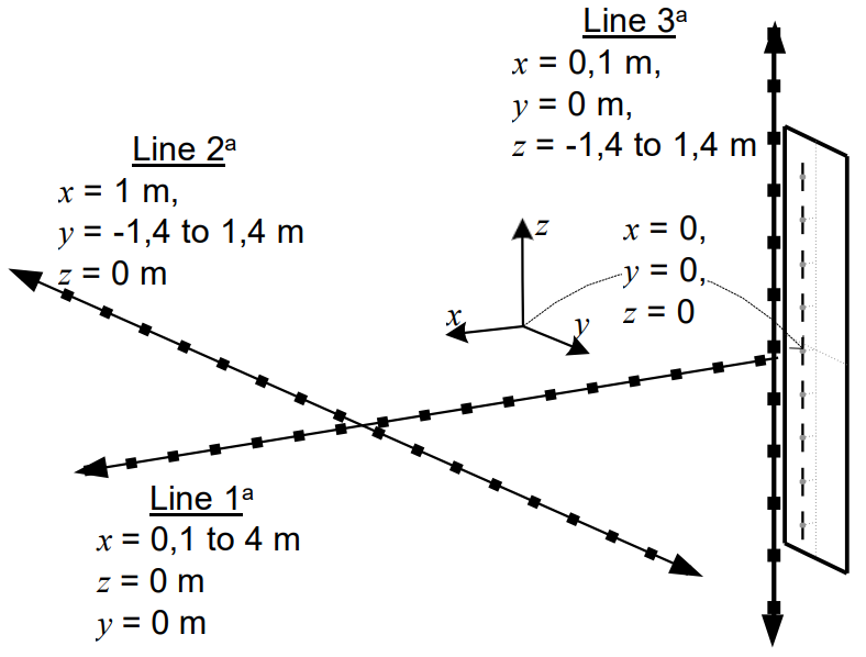
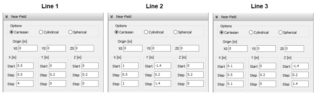
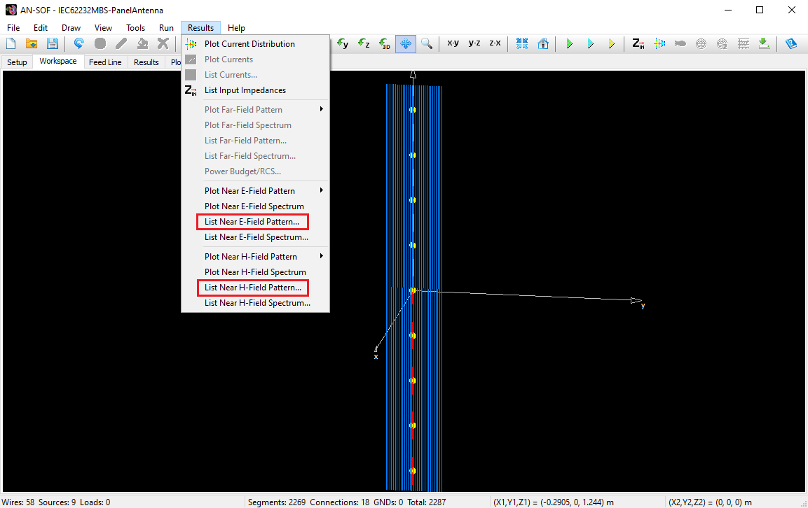
The near electric and magnetic fields generated by the antenna are evaluated along three distinct lines, as illustrated in Figure 2 of the IEC document. To compute these fields, the coordinates of the measurement points were input into the Near-Field panel panel in AN-SOF, as shown in Figure 3.
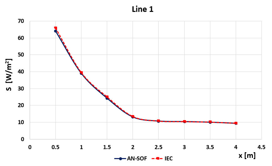
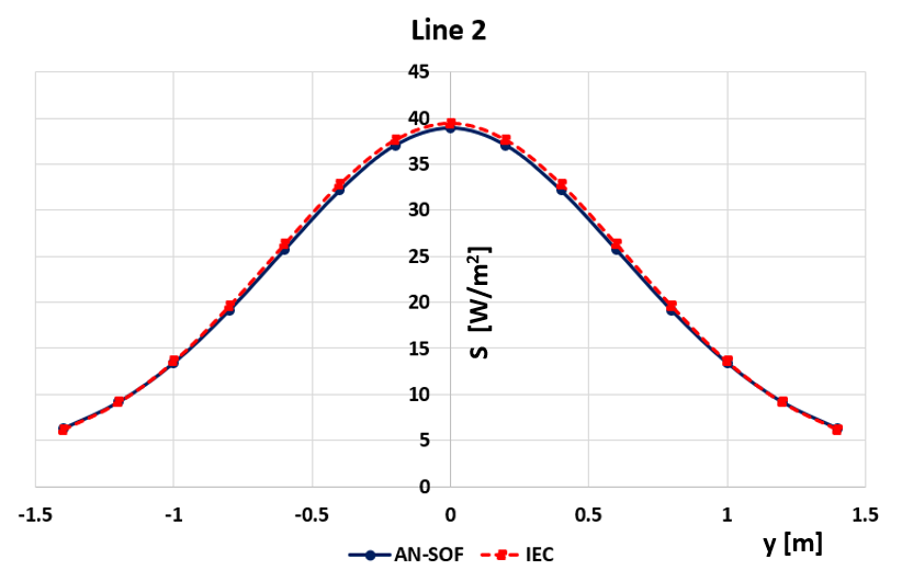
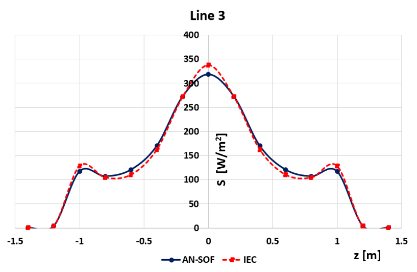
The IEC document provides reference tables detailing the power density ($S$, in W/m²) along these three lines. For a simulation tool to pass validation, the maximum deviation from the reference results must not exceed 10%.
Since all dipoles in the panel are vertically oriented, the radiated field exhibits vertical polarization. To accurately model the reflector panel in AN-SOF, a series of closely spaced vertical wires were employed, as illustrated in Figure 4. For optimal alignment with the IEC reference data, the reflector was modeled using 31 wires, each divided into 70 segments and assigned a radius of 0.1 mm.
Validation of Near-Field Power Density: AN-SOF vs. IEC Reference Results
The symmetry of the dipole array implies that the near electric field comprises two components, $E_x$ and $E_z$, while the near magnetic field consists solely of the $H_y$ component. The complex power density, $\mathbf{S}$, is derived from the vector product of the electric and magnetic fields (using RMS values):
$\displaystyle \mathbf{S} = \mathbf{E} \times \mathbf{H}^* \qquad (1)$
Consequently, $\mathbf{S}$ has two components:
$\displaystyle S_x = -E_z H_y^* \qquad (2)$
$\displaystyle S_z = +E_x H_y^* \qquad (3)$
The time-averaged power density, $S_{\text{tot}}$, is given by:
$\displaystyle S_{\text{tot}} = |\mathbf{S}| = \sqrt{\mathbf{S} \cdot \mathbf{S}^*} = \sqrt{|S_x|^2 + |S_z|^2} = \sqrt{|E_x|^2 + |E_z|^2} \,\, |H_y| \qquad (4)$
Thus,
$\displaystyle S_{\text{tot}} = E_{\text{tot}} \, H_{\text{tot}} \qquad (5)$
where $E_{\text{tot}} = \sqrt{|E_x|^2 + |E_z|^2}$ and $H_{\text{tot}} = |H_y|$ represent the RMS values of the total electric and magnetic fields, respectively. It is important to note that Equation (5) is not a general result but a special case arising from the orthogonality of the $\mathbf{E}$ and $\mathbf{H}$ fields, which is a direct consequence of the symmetry of this specific antenna geometry.
AN-SOF computes the RMS values of the total fields $E_{\text{tot}}$ and $H_{\text{tot}}$ as well as the RMS value of the total power density $S_{\text{tot}}$. The software allows users to tabulate, plot, and export the $\mathbf{E}$, $\mathbf{H}$, and $\mathbf{S}$ fields in the near-field region, with results available in CSV format for further analysis.
The tables and figures below compare the results obtained from AN-SOF with those published in the IEC document, where the reference values are derived using Equation (5). For all three measurement lines, the deviation between AN-SOF results and the IEC reference values is less than 10%. Notably, Lines 1 and 2 demonstrate an excellent fit to the IEC data. For Line 3, a slightly higher deviation is observed, which is expected due to the closer proximity of the measurement points to the antenna panel.
| X | Y | Z | E-total | H-total | AN-SOF | IEC | Diff. |
|---|---|---|---|---|---|---|---|
| m | m | m | V/m | A/m | W/m² | W/m² | % |
| 0.5 | 0 | 0 | 155.073 | 0.412721 | 64.0018 | 65.8 | -2.7% |
| 1 | 0 | 0 | 119.667 | 0.325309 | 38.9289 | 39.4 | -1.2% |
| 1.5 | 0 | 0 | 94.9649 | 0.254815 | 24.1985 | 25 | -3.2% |
| 2 | 0 | 0 | 70.7587 | 0.184969 | 13.0882 | 13.4 | -2.3% |
| 2.5 | 0 | 0 | 63.6878 | 0.167705 | 10.6808 | 10.7 | -0.18% |
| 3 | 0 | 0 | 62.4628 | 0.165972 | 10.3671 | 10.4 | -0.32% |
| 3.5 | 0 | 0 | 61.2367 | 0.163286 | 9.99912 | 10.1 | -1.0% |
| 4 | 0 | 0 | 59.1718 | 0.157914 | 9.34409 | 9.44 | -1.0% |
| X | Y | Z | E-total | H-total | AN-SOF | IEC | Diff. |
|---|---|---|---|---|---|---|---|
| m | m | m | V/m | A/m | W/m² | W/m² | % |
| 1 | -1.4 | 0 | 48.8216 | 0.129096 | 6.30268 | 6.22 | 1.3% |
| 1 | -1.2 | 0 | 58.5665 | 0.156658 | 9.17494 | 9.16 | 0.16% |
| 1 | -1 | 0 | 70.4701 | 0.190803 | 13.4459 | 13.6 | -1.1% |
| 1 | -0.8 | 0 | 83.6565 | 0.228631 | 19.1265 | 19.6 | -2.4% |
| 1 | -0.6 | 0 | 96.8025 | 0.265570 | 25.7078 | 26.3 | -2.3% |
| 1 | -0.4 | 0 | 108.375 | 0.296700 | 32.1548 | 32.8 | -2.0% |
| 1 | -0.2 | 0 | 116.618 | 0.317768 | 37.0575 | 37.6 | -1.4% |
| 1 | 0 | 0 | 119.667 | 0.325309 | 38.9289 | 39.4 | -1.2% |
| 1 | 0.2 | 0 | 116.618 | 0.317768 | 37.0575 | 37.6 | -1.4% |
| 1 | 0.4 | 0 | 108.375 | 0.296700 | 32.1548 | 32.8 | -2.0% |
| 1 | 0.6 | 0 | 96.8025 | 0.265570 | 25.7078 | 26.3 | -2.3% |
| 1 | 0.8 | 0 | 83.6565 | 0.228631 | 19.1265 | 19.6 | -2.4% |
| 1 | 1 | 0 | 70.4701 | 0.190803 | 13.4459 | 13.6 | -1.1% |
| 1 | 1.2 | 0 | 58.5665 | 0.156658 | 9.17494 | 9.16 | 0.2% |
| 1 | 1.4 | 0 | 48.8216 | 0.129096 | 6.30268 | 6.22 | 1.3% |
| X | Y | Z | E-total | H-total | AN-SOF | IEC | Diff. |
|---|---|---|---|---|---|---|---|
| m | m | m | V/m | A/m | W/m² | W/m² | % |
| 0.1 | 0 | -1.4 | 9.96449 | 0.0178238 | 0.177605 | 0.173 | 2.7% |
| 0.1 | 0 | -1.2 | 48.9680 | 0.0841207 | 4.11923 | 3.77 | 9.3% |
| 0.1 | 0 | -1 | 197.970 | 0.592135 | 117.225 | 129 | -9.1% |
| 0.1 | 0 | -0.8 | 201.216 | 0.532145 | 107.076 | 105 | 2.0% |
| 0.1 | 0 | -0.6 | 225.770 | 0.535062 | 120.801 | 111 | 8.8% |
| 0.1 | 0 | -0.4 | 268.066 | 0.634259 | 170.023 | 163 | 4.3% |
| 0.1 | 0 | -0.2 | 318.388 | 0.855278 | 272.310 | 272 | 0.11% |
| 0.1 | 0 | 0 | 337.217 | 0.944107 | 318.369 | 338 | -5.8% |
| 0.1 | 0 | 0.2 | 318.388 | 0.855278 | 272.310 | 272 | 0.11% |
| 0.1 | 0 | 0.4 | 268.066 | 0.634259 | 170.023 | 163 | 4.3% |
| 0.1 | 0 | 0.6 | 225.770 | 0.535062 | 120.801 | 111 | 8.8% |
| 0.1 | 0 | 0.8 | 201.216 | 0.532145 | 107.076 | 105 | 2.0% |
| 0.1 | 0 | 1 | 197.970 | 0.592135 | 117.225 | 129 | -9.1% |
| 0.1 | 0 | 1.2 | 48.9680 | 0.0841207 | 4.11923 | 3.77 | 9.3% |
| 0.1 | 0 | 1.4 | 9.96449 | 0.0178238 | 0.177605 | 0.173 | 2.7% |
Conclusion
The successful validation of AN-SOF against the IEC 62232 standard highlights the software’s ability to produce highly accurate results, even when using a relatively simple antenna model. This achievement not only demonstrates AN-SOF’s computational precision but also reinforces its reliability in adhering to international standards. Such validation is critical for engineers, researchers, and regulatory bodies who rely on accurate simulations to evaluate compliance with safety guidelines and optimize antenna designs.
