Search for answers or browse our Knowledge Base.
Guides | Models | Validation | Book
Radar Cross Section and Reception Characteristics of a Passive Loop Antenna: A Simulation Study
This article analyzes radar cross section (RCS) and reception properties of a passive loop antenna via full-wave simulation. We demonstrate how loop resonance manifests in both RCS patterns and load voltage characteristics.
Understanding Radar Cross Section (RCS) Through Loop Antenna Modeling
Radar Cross Section (RCS) is a fundamental metric in electromagnetics that quantifies how detectable an object is when illuminated by a radar signal. Expressed in square meters, RCS describes the effective area that intercepts and scatters incident electromagnetic energy back toward the radar receiver. While RCS is most commonly associated with stealth technology and military applications—where minimizing detectability is critical—it also plays a significant role in antenna design, particularly in scenarios where unintended scattering or interference must be considered.
In this article, we’ll examine the RCS of a loop antenna, demonstrating how simulation helps visualize and quantify its scattering characteristics. Whether you’re an RF professional optimizing antenna stealth, a ham radio operator mitigating interference, or an academic researcher exploring electromagnetic theory, understanding RCS enriches our grasp of how antennas interact with their environment beyond mere transmission and reception. Let’s dive in!
Simulating a Receiving Loop Antenna for RCS Analysis
To demonstrate Radar Cross Section (RCS) principles, we’ll model a circular loop antenna operating in reception mode. Unlike a transmitting antenna, this passive structure is not driven by a discrete source or generator. Instead, it interacts with an incoming plane wave, inducing a measurable voltage across a terminating 50-ohm load impedance. This configuration allows us to examine two key behaviors simultaneously: the antenna’s scattering characteristics (RCS) and its performance as a receiver.
Defining the Antenna Geometry
The model consists of a one-meter diameter loop (radius = 0.5 m) centered at the origin (0,0,0). In AN-SOF, we begin by selecting Circle from the Draw menu and specifying the center coordinates and radius (Fig. 1a). The loop’s orientation is set by defining its normal vector along the +Y-axis through spherical coordinates (Theta = 90°, Phi = 90°), which positions the loop on the XZ-plane (Fig. 1b).
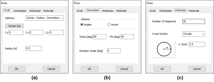
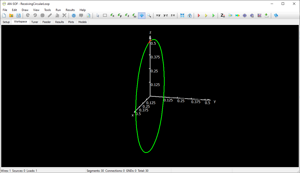
For accurate simulation, we configure the wire properties with 30 segments around the circumference and assign a circular cross-section with a 2.5 mm radius (Fig. 1c). This discretization ensures smooth current distribution while maintaining computational efficiency. The completed structure appears in the workspace as shown in Figure 2.
Configuring the Load and Excitation
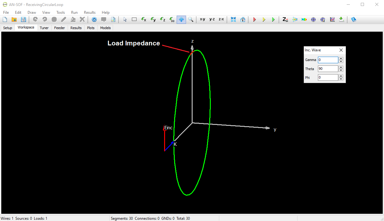
To model the receiving behavior, we terminate the loop with a 50-ohm load at its topmost point. This is done by right-clicking the loop, selecting Source/Load/TL, and precisely placing the load using the interactive slider.
The frequency sweep is set from 40 to 140 MHz in 1 MHz increments. This range is chosen to capture the loop’s first resonance and associated RCS variations. The incident plane wave is defined in the Excitation panel, where we specify the propagation direction (Theta, Phi) and polarization angle (Gamma). For optimal energy transfer, we align the wave’s electric field vector parallel to the loop plane, ensuring the magnetic field is normal to it as illustrated in Figure 3.
Executing the Simulation
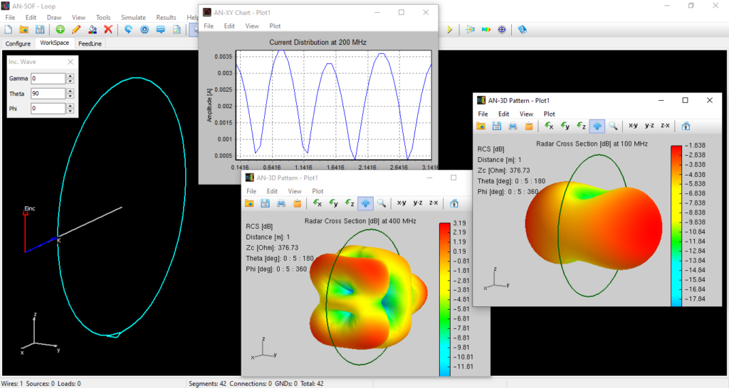
With all parameters configured, we initiate the computation by clicking Run Currents and Far-Field (F10). This generates three key results: the induced current distribution along the loop conductor, the received voltage across the load, and the far-field scattering pattern that defines the RCS.
The next section will analyze these results in detail, focusing on the relationship between reception efficiency and scattering behavior across the frequency spectrum. We’ll particularly examine how structural resonance affects both the received signal strength and the antenna’s detectability via its RCS profile.
Analyzing RCS Behavior and Resonance Effects in the Loop Antenna
3D RCS Patterns and Frequency Dependence
The most visually striking result of our simulation is the three-dimensional RCS pattern, which reveals how the loop antenna scatters incident energy across different frequencies. To visualize the antenna’s scattering behavior, we generate a 3D directional RCS pattern by clicking Far-Field 3D Plot in the toolbar and selecting Plot > RCS > Total. Figure 4 shows an animated representation of how the RCS varies across the 40–140 MHz frequency range, revealing key changes in magnitude and lobe structure.
At the lower end of our frequency range (40 MHz), where the loop circumference (π ≈ 3.14 m) is about 0.4λ, the scattered field exhibits a single dominant lobe in the +X direction—the same axis as the incoming wave. This behavior is characteristic of electrically small loops, which act primarily as magnetic dipoles.
As frequency increases, two key phenomena emerge:
- Magnitude Variation: The peak RCS grows from just 0.019 m² at 40 MHz to a sharp maximum of 5.9 m² at 100 MHz—the frequency where the loop’s circumference equals one wavelength (1λ). Beyond this point, RCS declines rapidly, falling to 0.22 m² at 140 MHz.
- Directional Shifts: The angular distribution of scattered energy undergoes dramatic changes. At resonance (100 MHz), the RCS peak splits into dual lobes along the ±Y axis, while at higher frequencies, the maxima reorient along the Z axis.
The Resonance Connection: RCS and Receive Voltage
The RCS peak at 100 MHz is no coincidence—it aligns precisely with the loop’s natural resonant frequency as a transmitting antenna. Figure 5a plots the RCS versus frequency, generated via AN-SOF Main Menu > Results > Power Budget/RCS. This correlation is further evidenced by the load voltage characteristics (Figure 5b). To extract these values, right-click the loop, select List Currents, and locate the load position to view the frequency-dependent voltage across the 50-Ω termination.
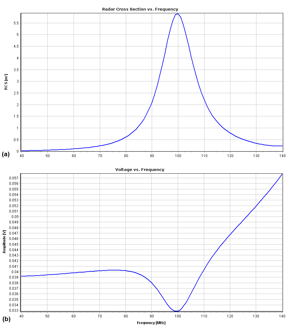
A striking pattern emerges:
- The RCS maximum at 100 MHz coincides exactly with a minimum in load voltage.
- This inverse correlation occurs because at resonance, the loop efficiently reradiates intercepted energy rather than delivering it to the load.
Practical Implications and Measurement Techniques
These results highlight two critical insights:
- RCS Predictability: The strong coupling between RCS peaks and impedance resonance means that simple voltage measurements at a load can serve as a proxy for estimating scattering behavior—a valuable shortcut for stealth or interference-sensitive applications.
- Frequency-Dependent Stealth: For systems where low detectability is paramount, operating away from the loop’s resonant frequency (here, 100 MHz) significantly reduces radar visibility.
Conclusion: A Unified View of Reception and Scattering
This analysis bridges the often-separated domains of antenna reception and radar signature. The loop’s behavior demonstrates that:
- Resonance governs both RCS and receive performance, but with opposing optima.
- 3D scattering patterns provide intuitive diagnostics for antenna detectability.
- Load measurements offer a practical way to infer RCS properties without full-wave simulations.
