Search for answers or browse our Knowledge Base.
Guides | Models | Validation | Book
Circuit Theory Validation: Simulating an RLC Series Resonator
Validate the high-precision numerical stability of AN-SOF at the extreme low-frequency limit. This article details a simulation of a series RLC circuit designed to resonate at 800 Hz, where the wavelength is 375 kilometers. By comparing the simulated current peaks against classical circuit theory formulas, we demonstrate that the AN-SOF engine maintains its accuracy even when the structure size is a minute fraction of the wavelength. This study provides a step-by-step validation of lumped-element integration and frequency-sweep stability for complex system modeling.
Introduction to Low-Frequency Numerical Stability
The Method of Moments (MoM) is traditionally utilized for the analysis of antennas and scatterers at frequencies where the structure size is comparable to the wavelength. However, a significant benchmark for a robust electromagnetic solver is its ability to remain numerically stable in the low-frequency limit. When the operating frequency is extremely low, the wavelength becomes enormous relative to the antenna geometry, often leading to precision issues known as “low-frequency breakdown” in many simulation engines.
This article details the validation of AN-SOF against classical circuit theory by modeling a series RLC circuit. The simulation is conducted at $800 \text{ Hz}$, a frequency where the wavelength is approximately $375$ kilometers. By successfully capturing the resonant behavior of a millimeter-scale circuit at this scale, we demonstrate that the AN-SOF engine maintains its accuracy and dynamic range across vastly different orders of magnitude.
Simulation Setup and Configuration
To replicate a circuit-theory environment, the units of measurement must be adjusted to suit lumped component values. The first step involves navigating to Tools > Preferences to select $\text{Hz}$ for frequency, $\text{mm}$ for length, $\text{mH}$ for inductance, and $\mu\text{F}$ for capacitance.
Frequency and Environment Parameters
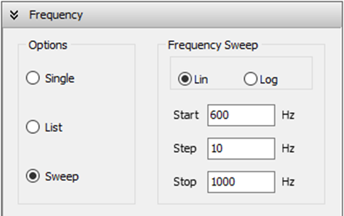
The simulation is configured as a linear frequency sweep to identify the resonant peak. As shown in Fig. 1(a), the sweep starts at $600 \text{ Hz}$ and terminates at $1,000 \text{ Hz}$ with a step size of $10 \text{ Hz}$. To provide a reference for the return path of the circuit, a perfect ground plane is established at $z = 0$, as illustrated in Fig. 1(b). This environment ensures that the calculated impedances are referenced to a consistent potential, mirroring the “ground” node in a standard schematic.

Geometric Representation and Lumped Elements
The physical model consists of three interconnected wires that form a small loop, as shown in the workspace coordinates for Fig. 2. In this validation, the “wires” do not act as efficient radiators because their physical length is an infinitesimal fraction of the $375 \text{ km}$ wavelength. Instead, they serve as the physical carriers for lumped $R$, $L$, and $C$ components.
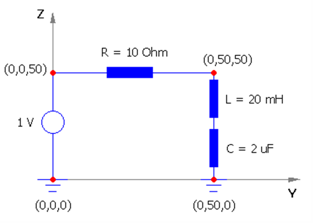
In AN-SOF, these components are integrated directly into the wire segments. A voltage source is applied to the first segment to drive the circuit, while the resistive, inductive, and capacitive properties are defined as lumped loads. This allows the Method of Moments to solve for the current distribution based on both the geometric properties of the wire and the mathematical constraints of the lumped elements.
Analysis of Current and Resonance
Once the simulation is executed, the current distribution is analyzed across the three wires. Because this is a series configuration, the current amplitude must remain identical in all segments, a fact that is easily verified using the List Currents command in the AN-SOF interface.
Figure 3 displays the plot of current amplitude versus frequency. The curve shows a distinct, sharp peak that characterizes a high-Q series resonator. According to standard circuit theory, the resonant frequency ($f_r$) of a series RLC circuit is determined by:
$\displaystyle f_r \,=\, \frac{1}{2\pi\sqrt{LC}}$
By substituting the values for $L$ and $C$, we get:
$\displaystyle f_r \,=\, \frac{1}{2 \pi \sqrt{20 \times 10^{-3} \times 2 \times 10^{-6}}} \,\approx\, 796 \text{ Hz}$
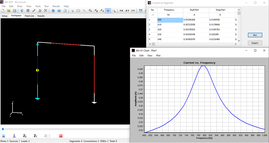
The simulation results plotted in Fig. 3 show that the peak current occurs exactly near the $800 \text{ Hz}$ mark. In fact, by zooming in on the plot around $800 \text{ Hz}$, it can be verified that the resonance frequency obtained from the simulation is $796 \text{ Hz}$, agreeing with the theory to three significant figures. This aligns extremely well with the theoretical prediction based on the values of the lumped components used in the model. The ability of the software to pinpoint this peak at such a low frequency confirms the stability of the exact kernel implemented in AN-SOF.
Conclusion
The successful modeling of an RLC circuit at 800 Hz serves as a definitive validation of AN-SOF’s numerical methods. By producing results that match classical circuit theory formulas, the simulation proves that the engine does not suffer from the precision loss or “zero-frequency” singularities that plague many other MoM-based tools.
The convergence of the current amplitude at the predicted 800 Hz resonant frequency (Fig. 3) demonstrates that the software can effectively bridge the gap between full-wave electromagnetics and lumped-element circuit analysis. This implies that AN-SOF is capable of simulating complex systems that include both radiating elements and low-frequency matching networks or filter components, providing a single, unified environment for high-precision RF and low-frequency design.
See Also:
Technical Keywords: RLC Circuit Simulation, Low-Frequency Stability, Circuit Theory Validation, Resonant Frequency, Lumped Elements, AN-SOF Numerical Methods, Frequency Sweep, Current Amplitude, Exact Kernel.
